Street Networks & Web Scraping

Part 1: Visualizing crash data in Philadelphia

In this section, you will use osmnx to analyze the crash incidence in Center City.

Part 2: Scraping Craigslist

In this section, you will use Selenium and BeautifulSoup to scrape data for hundreds of apartments from Philadelphia’s Craigslist portal.

Part 1: Visualizing crash data in Philadelphia

1.1 Load the geometry for the region being analyzed We’ll analyze crashes in the “Central” planning district in Philadelphia, a rough approximation for Center City. Planning districts can be loaded from Open Data Philly. Read the data into a GeoDataFrame using the following link:

http://data.phl.opendata.arcgis.com/datasets/0960ea0f38f44146bb562f2b212075aa_0.geojson

Select the “Central” district and extract the geometry polygon for only this district. After this part, you should have a polygon variable of type shapely.geometry.polygon.Polygon

import pandas as pd
import geopandas as gpd
import numpy as np
import hvplot.pandas 
import altair as alt
import matplotlib.pyplot as plt
import rasterio as rio
import osmnx as ox
pd.options.display.max_columns = 999

# Hide warnings due to issue in shapely package 
# See: https://github.com/shapely/shapely/issues/1345
np.seterr(invalid="ignore");

CPD = gpd.read_file("http://data.phl.opendata.arcgis.com/datasets/0960ea0f38f44146bb562f2b212075aa_0.geojson")
#CPD = ox.geocode_to_gdf("http://data.phl.opendata.arcgis.com/datasets/0960ea0f38f44146bb562f2b212075aa_0.geojson")
CPD = CPD[CPD["ABBREV"] == "CTR"]
CPD

	OBJECTID_1	OBJECTID	DIST_NAME	ABBREV	Shape__Area	Shape__Length	PlanningDist	DaytimePop	geometry
3	4	9	Central	CTR	1.782880e+08	71405.14345	NaN	NaN	POLYGON ((-75.14791 39.96733, -75.14715 39.967...

Phillyox = ox.geocode_to_gdf("Philadelphia, PA")
Phillyox.crs

<Geographic 2D CRS: EPSG:4326>
Name: WGS 84
Axis Info [ellipsoidal]:
- Lat[north]: Geodetic latitude (degree)
- Lon[east]: Geodetic longitude (degree)
Area of Use:
- name: World.
- bounds: (-180.0, -90.0, 180.0, 90.0)
Datum: World Geodetic System 1984 ensemble
- Ellipsoid: WGS 84
- Prime Meridian: Greenwich

1.2 Get the street network graph

Use OSMnx to create a network graph (of type ‘drive’) from your polygon boundary in 1.1.

ax = ox.project_gdf(CPD).plot(fc="lightgreen", ec="black")
ax.set_axis_off()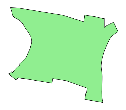

ax = CPD.to_crs(epsg=2272).plot(facecolor="none", edgecolor="black")
ax.set_axis_off()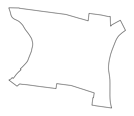

streets = ox.features_from_place("Philadelphia, PA", tags={"highway": True})

streets.head(6)

		highway	geometry	traffic_signals	traffic_signals:direction	railway	crossing	ref	noref	noexit	ref:left	ref:right	old_ref	disused:railway	stop	name	crossing:markings	direction	traffic_calming	tactile_paving	access	source	crossing_ref	bicycle	description	foot	horse	motor_vehicle	addr:city	addr:housenumber	addr:postcode	addr:state	addr:street	website	note	crossing:island	proposed:junction	supervised	except	proposed:highway	ford	ele	gnis:feature_id	bench	bus	covered	network	network:wikidata	operator	public_transport	shelter	kerb	junction	gate	parking	wheelchair	network:wikipedia	indoor	level	fixme	route_ref	local_ref	designation	leisure	aeroway	maxheight	heritage	heritage:operator	ref:nrhp	material	bin	lit	traffic_signals:sound	lamp_type	departures_board	capacity	button_operated	layer	opening_hours	surface	traffic_signals:vibration	internet_access	route_ref_1	landuse	alt_name	lamp_mount	traffic_sign	operator:wikidata	short_name	brand	brand:wikidata	tram	motor_vehicle:conditional	hgv	tourism	trolleybus	network:short	man_made	flashing_lights	abandoned	not:network:wikidata	support	traffic_signals:countdown	historic	cycleway	informal	advertising	check_date:crossing	nodes	oneway	tiger:cfcc	tiger:name_base	tiger:name_type	tiger:reviewed	tiger:zip_left	tiger:zip_right	lane_markings	lanes	tiger:name_direction_prefix	tiger:separated	tiger:source	tiger:tlid	tiger:zip_left_1	service	parking:lane:both	sidewalk	cycleway:right	old_ref_legislative	ref:penndot	tiger:name_direction_suffix	destination:ref	turn:lanes	destination	toll	destination:ref:to	maxspeed	source:hgv	source:ref:penndot	smoothness	bridge	junction:ref	destination:lanes	width	cycleway:both	cycleway:both:buffer	NHS	cycleway:right:buffer	check_date:smoothness	destination:street	wikipedia	lanes:backward	lanes:forward	turn:lanes:backward	tracktype	turn	maxspeed:advisory	psv	destination:symbol	tunnel	noname	maxweight:signed	tiger:name_base_1	source:width	rcn_ref	abandoned:railway	parking:lane:left	parking:lane:left:parallel	parking:lane:right	cycleway:left	embedded_rails	name_1	tiger:name_base_2	tiger:name_type_1	destination:ref:lanes	old_ref:legislative	destination:to	tiger:zip_left_2	tiger:zip_right_1	tiger:zip_right_2	cycleway:left:buffer	cycleway:right:lane	source:oneway	sidewalk:both	lcn	parking:lane:right:parallel	maxspeed:type	parking:both	parking:orientation	sidewalk:both:surface	centre_turn_lane	tiger:zip_left_3	tiger:zip_left_4	parking:left	parking:right	parking:right:orientation	sidewalk:left	sidewalk:right	maxwidth	old_name	maxspeed:backward	old_railway_operator	bicycle:backward:conditional	bicycle:forward:conditional	name:etymology:wikidata	oneway:bicycle	construction	wikidata	incline	check_date:surface	destination:street:lanes	parking:both:orientation	access:hgv	maxweight	FIXME	lanes:both_ways	turn:lanes:both_ways	turn:lanes:forward	tiger:zip_right_3	source:lanes	restriction:hgv	maxspeed:forward	tiger:name_direction_prefix_1	parking:lane:both:parallel	note:lanes	name_2	tiger:name_direction_prefix_2	tiger:name_type_2	tiger:zip_right_4	motorcar	tiger:name_direction	note:old_railway_operator	toll:backward	toll:forward	bicycle:forward	parking:condition:right	bicycle:backward	maxwidth:physical	tiger:name_base_3	tiger:name_direction_prefix_3	tiger:name_type_3	source:boundary	segregated	bridge:name	start_date	name2	created_by	motorroad	footway	maxspeed:variable	tiger:county	destination:ref:to:lanes	area	handrail	ramp	parking:left:markings	parking:left:orientation	step_count	sac_scale	trail_visibility	trolley_wire	voltage	highspeed	check_date	base_material_values	bridge:structure	embankment	destination:lanes:forward	destination:ref:to:lanes:forward	destination:ref:lanes:forward	destination:ref:to:lanes:backward	disused:cycleway:both	destination:lanes:backward	opening_date	lanes:bus	mtb:scale	access:lanes:forward	psv:lanes:forward	placement:backward	canoe	surface:condition	destination:ref:forward	destination:street:forward	tiger:zip	unsigned_ref	hgv:lanes	shoulder	placement	abandoned:highway	destination:ref:lanes:backward	proposed	bicycle:lane	loc_name	ramp:wheelchair	mtb:scale:imba	mtb:scale:uphill	disused:cycleway:right	goods	cutting	cycleway:left:oneway	parking:condition:left	parking:condition:left:time_interval	ski	snowmobile	emergency	source:name	name:en	HFCS	NJDOT_SRI	bridge:movable	hgv:state_network	source:hgv:state_network	change:lanes:backward	change:lanes:forward	parking:lane:right:diagonal	levels	postal_code	location	length	sport	closed	condition	danger	danger_1	hazard	cycleway:both:width	parking:lane:left:diagonal	PARK_NAME	SHAPE_LENG	TRL_LENGTH	parking:condition:both	proposed:lanes	proposed:lanes:forward	proposed:turn:lanes:forward	proposed:lanes:backward	proposed:turn:lanes:backward	placement:forward	destination:street:backward	destination:street:lanes:forward	destination:street:lanes:backward	name:backward	name:forward	cycleway:buffer	turn:backward	golf	gauge	parking:condition:both:time_interval	train	horse_scale	dog	turn:forward	surface:lanes:backward	surface:lanes:forward	bus:backward	hgv:backward	motorcar:backward	motorroad:backward	artist:website	artist:wikidata	artist_name	not:name	golf_cart	steps	comment	historic:railway	disused:cycleway:left	oneway:bus	stairs	sidewalk:left:surface	sidewalk:right:surface	truck	stroller	conveying	check_date:handrail	ways	type
element_type	osmid
node	109727831	traffic_signals	POINT (-75.15328 40.02996)	NaN	NaN	NaN	NaN	NaN	NaN	NaN	NaN	NaN	NaN	NaN	NaN	NaN	NaN	NaN	NaN	NaN	NaN	NaN	NaN	NaN	NaN	NaN	NaN	NaN	NaN	NaN	NaN	NaN	NaN	NaN	NaN	NaN	NaN	NaN	NaN	NaN	NaN	NaN	NaN	NaN	NaN	NaN	NaN	NaN	NaN	NaN	NaN	NaN	NaN	NaN	NaN	NaN	NaN	NaN	NaN	NaN	NaN	NaN	NaN	NaN	NaN	NaN	NaN	NaN	NaN	NaN	NaN	NaN	NaN	NaN	NaN	NaN	NaN	NaN	NaN	NaN	NaN	NaN	NaN	NaN	NaN	NaN	NaN	NaN	NaN	NaN	NaN	NaN	NaN	NaN	NaN	NaN	NaN	NaN	NaN	NaN	NaN	NaN	NaN	NaN	NaN	NaN	NaN	NaN	NaN	NaN	NaN	NaN	NaN	NaN	NaN	NaN	NaN	NaN	NaN	NaN	NaN	NaN	NaN	NaN	NaN	NaN	NaN	NaN	NaN	NaN	NaN	NaN	NaN	NaN	NaN	NaN	NaN	NaN	NaN	NaN	NaN	NaN	NaN	NaN	NaN	NaN	NaN	NaN	NaN	NaN	NaN	NaN	NaN	NaN	NaN	NaN	NaN	NaN	NaN	NaN	NaN	NaN	NaN	NaN	NaN	NaN	NaN	NaN	NaN	NaN	NaN	NaN	NaN	NaN	NaN	NaN	NaN	NaN	NaN	NaN	NaN	NaN	NaN	NaN	NaN	NaN	NaN	NaN	NaN	NaN	NaN	NaN	NaN	NaN	NaN	NaN	NaN	NaN	NaN	NaN	NaN	NaN	NaN	NaN	NaN	NaN	NaN	NaN	NaN	NaN	NaN	NaN	NaN	NaN	NaN	NaN	NaN	NaN	NaN	NaN	NaN	NaN	NaN	NaN	NaN	NaN	NaN	NaN	NaN	NaN	NaN	NaN	NaN	NaN	NaN	NaN	NaN	NaN	NaN	NaN	NaN	NaN	NaN	NaN	NaN	NaN	NaN	NaN	NaN	NaN	NaN	NaN	NaN	NaN	NaN	NaN	NaN	NaN	NaN	NaN	NaN	NaN	NaN	NaN	NaN	NaN	NaN	NaN	NaN	NaN	NaN	NaN	NaN	NaN	NaN	NaN	NaN	NaN	NaN	NaN	NaN	NaN	NaN	NaN	NaN	NaN	NaN	NaN	NaN	NaN	NaN	NaN	NaN	NaN	NaN	NaN	NaN	NaN	NaN	NaN	NaN	NaN	NaN	NaN	NaN	NaN	NaN	NaN	NaN	NaN	NaN	NaN	NaN	NaN	NaN	NaN	NaN	NaN	NaN	NaN	NaN	NaN	NaN	NaN	NaN	NaN	NaN	NaN	NaN	NaN	NaN	NaN	NaN	NaN	NaN	NaN	NaN	NaN	NaN	NaN	NaN	NaN	NaN	NaN	NaN	NaN	NaN	NaN	NaN	NaN	NaN	NaN	NaN	NaN	NaN	NaN	NaN	NaN	NaN	NaN	NaN	NaN	NaN	NaN	NaN	NaN	NaN	NaN	NaN	NaN	NaN	NaN	NaN	NaN	NaN
	109727914	traffic_signals	POINT (-75.13837 40.02803)	signal	NaN	NaN	NaN	NaN	NaN	NaN	NaN	NaN	NaN	NaN	NaN	NaN	NaN	NaN	NaN	NaN	NaN	NaN	NaN	NaN	NaN	NaN	NaN	NaN	NaN	NaN	NaN	NaN	NaN	NaN	NaN	NaN	NaN	NaN	NaN	NaN	NaN	NaN	NaN	NaN	NaN	NaN	NaN	NaN	NaN	NaN	NaN	NaN	NaN	NaN	NaN	NaN	NaN	NaN	NaN	NaN	NaN	NaN	NaN	NaN	NaN	NaN	NaN	NaN	NaN	NaN	NaN	NaN	NaN	NaN	NaN	NaN	NaN	NaN	NaN	NaN	NaN	NaN	NaN	NaN	NaN	NaN	NaN	NaN	NaN	NaN	NaN	NaN	NaN	NaN	NaN	NaN	NaN	NaN	NaN	NaN	NaN	NaN	NaN	NaN	NaN	NaN	NaN	NaN	NaN	NaN	NaN	NaN	NaN	NaN	NaN	NaN	NaN	NaN	NaN	NaN	NaN	NaN	NaN	NaN	NaN	NaN	NaN	NaN	NaN	NaN	NaN	NaN	NaN	NaN	NaN	NaN	NaN	NaN	NaN	NaN	NaN	NaN	NaN	NaN	NaN	NaN	NaN	NaN	NaN	NaN	NaN	NaN	NaN	NaN	NaN	NaN	NaN	NaN	NaN	NaN	NaN	NaN	NaN	NaN	NaN	NaN	NaN	NaN	NaN	NaN	NaN	NaN	NaN	NaN	NaN	NaN	NaN	NaN	NaN	NaN	NaN	NaN	NaN	NaN	NaN	NaN	NaN	NaN	NaN	NaN	NaN	NaN	NaN	NaN	NaN	NaN	NaN	NaN	NaN	NaN	NaN	NaN	NaN	NaN	NaN	NaN	NaN	NaN	NaN	NaN	NaN	NaN	NaN	NaN	NaN	NaN	NaN	NaN	NaN	NaN	NaN	NaN	NaN	NaN	NaN	NaN	NaN	NaN	NaN	NaN	NaN	NaN	NaN	NaN	NaN	NaN	NaN	NaN	NaN	NaN	NaN	NaN	NaN	NaN	NaN	NaN	NaN	NaN	NaN	NaN	NaN	NaN	NaN	NaN	NaN	NaN	NaN	NaN	NaN	NaN	NaN	NaN	NaN	NaN	NaN	NaN	NaN	NaN	NaN	NaN	NaN	NaN	NaN	NaN	NaN	NaN	NaN	NaN	NaN	NaN	NaN	NaN	NaN	NaN	NaN	NaN	NaN	NaN	NaN	NaN	NaN	NaN	NaN	NaN	NaN	NaN	NaN	NaN	NaN	NaN	NaN	NaN	NaN	NaN	NaN	NaN	NaN	NaN	NaN	NaN	NaN	NaN	NaN	NaN	NaN	NaN	NaN	NaN	NaN	NaN	NaN	NaN	NaN	NaN	NaN	NaN	NaN	NaN	NaN	NaN	NaN	NaN	NaN	NaN	NaN	NaN	NaN	NaN	NaN	NaN	NaN	NaN	NaN	NaN	NaN	NaN	NaN	NaN	NaN	NaN	NaN	NaN	NaN	NaN	NaN	NaN	NaN	NaN	NaN	NaN	NaN	NaN	NaN	NaN	NaN	NaN	NaN	NaN	NaN	NaN	NaN	NaN	NaN	NaN	NaN
	109727992	traffic_signals	POINT (-75.14616 40.02904)	signal	NaN	NaN	NaN	NaN	NaN	NaN	NaN	NaN	NaN	NaN	NaN	NaN	NaN	NaN	NaN	NaN	NaN	NaN	NaN	NaN	NaN	NaN	NaN	NaN	NaN	NaN	NaN	NaN	NaN	NaN	NaN	NaN	NaN	NaN	NaN	NaN	NaN	NaN	NaN	NaN	NaN	NaN	NaN	NaN	NaN	NaN	NaN	NaN	NaN	NaN	NaN	NaN	NaN	NaN	NaN	NaN	NaN	NaN	NaN	NaN	NaN	NaN	NaN	NaN	NaN	NaN	NaN	NaN	NaN	NaN	NaN	NaN	NaN	NaN	NaN	NaN	NaN	NaN	NaN	NaN	NaN	NaN	NaN	NaN	NaN	NaN	NaN	NaN	NaN	NaN	NaN	NaN	NaN	NaN	NaN	NaN	NaN	NaN	NaN	NaN	NaN	NaN	NaN	NaN	NaN	NaN	NaN	NaN	NaN	NaN	NaN	NaN	NaN	NaN	NaN	NaN	NaN	NaN	NaN	NaN	NaN	NaN	NaN	NaN	NaN	NaN	NaN	NaN	NaN	NaN	NaN	NaN	NaN	NaN	NaN	NaN	NaN	NaN	NaN	NaN	NaN	NaN	NaN	NaN	NaN	NaN	NaN	NaN	NaN	NaN	NaN	NaN	NaN	NaN	NaN	NaN	NaN	NaN	NaN	NaN	NaN	NaN	NaN	NaN	NaN	NaN	NaN	NaN	NaN	NaN	NaN	NaN	NaN	NaN	NaN	NaN	NaN	NaN	NaN	NaN	NaN	NaN	NaN	NaN	NaN	NaN	NaN	NaN	NaN	NaN	NaN	NaN	NaN	NaN	NaN	NaN	NaN	NaN	NaN	NaN	NaN	NaN	NaN	NaN	NaN	NaN	NaN	NaN	NaN	NaN	NaN	NaN	NaN	NaN	NaN	NaN	NaN	NaN	NaN	NaN	NaN	NaN	NaN	NaN	NaN	NaN	NaN	NaN	NaN	NaN	NaN	NaN	NaN	NaN	NaN	NaN	NaN	NaN	NaN	NaN	NaN	NaN	NaN	NaN	NaN	NaN	NaN	NaN	NaN	NaN	NaN	NaN	NaN	NaN	NaN	NaN	NaN	NaN	NaN	NaN	NaN	NaN	NaN	NaN	NaN	NaN	NaN	NaN	NaN	NaN	NaN	NaN	NaN	NaN	NaN	NaN	NaN	NaN	NaN	NaN	NaN	NaN	NaN	NaN	NaN	NaN	NaN	NaN	NaN	NaN	NaN	NaN	NaN	NaN	NaN	NaN	NaN	NaN	NaN	NaN	NaN	NaN	NaN	NaN	NaN	NaN	NaN	NaN	NaN	NaN	NaN	NaN	NaN	NaN	NaN	NaN	NaN	NaN	NaN	NaN	NaN	NaN	NaN	NaN	NaN	NaN	NaN	NaN	NaN	NaN	NaN	NaN	NaN	NaN	NaN	NaN	NaN	NaN	NaN	NaN	NaN	NaN	NaN	NaN	NaN	NaN	NaN	NaN	NaN	NaN	NaN	NaN	NaN	NaN	NaN	NaN	NaN	NaN	NaN	NaN	NaN	NaN	NaN	NaN	NaN	NaN	NaN	NaN	NaN	NaN	NaN
	109727997	traffic_signals	POINT (-75.14686 40.02914)	NaN	NaN	NaN	NaN	NaN	NaN	NaN	NaN	NaN	NaN	NaN	NaN	NaN	NaN	NaN	NaN	NaN	NaN	NaN	NaN	NaN	NaN	NaN	NaN	NaN	NaN	NaN	NaN	NaN	NaN	NaN	NaN	NaN	NaN	NaN	NaN	NaN	NaN	NaN	NaN	NaN	NaN	NaN	NaN	NaN	NaN	NaN	NaN	NaN	NaN	NaN	NaN	NaN	NaN	NaN	NaN	NaN	NaN	NaN	NaN	NaN	NaN	NaN	NaN	NaN	NaN	NaN	NaN	NaN	NaN	NaN	NaN	NaN	NaN	NaN	NaN	NaN	NaN	NaN	NaN	NaN	NaN	NaN	NaN	NaN	NaN	NaN	NaN	NaN	NaN	NaN	NaN	NaN	NaN	NaN	NaN	NaN	NaN	NaN	NaN	NaN	NaN	NaN	NaN	NaN	NaN	NaN	NaN	NaN	NaN	NaN	NaN	NaN	NaN	NaN	NaN	NaN	NaN	NaN	NaN	NaN	NaN	NaN	NaN	NaN	NaN	NaN	NaN	NaN	NaN	NaN	NaN	NaN	NaN	NaN	NaN	NaN	NaN	NaN	NaN	NaN	NaN	NaN	NaN	NaN	NaN	NaN	NaN	NaN	NaN	NaN	NaN	NaN	NaN	NaN	NaN	NaN	NaN	NaN	NaN	NaN	NaN	NaN	NaN	NaN	NaN	NaN	NaN	NaN	NaN	NaN	NaN	NaN	NaN	NaN	NaN	NaN	NaN	NaN	NaN	NaN	NaN	NaN	NaN	NaN	NaN	NaN	NaN	NaN	NaN	NaN	NaN	NaN	NaN	NaN	NaN	NaN	NaN	NaN	NaN	NaN	NaN	NaN	NaN	NaN	NaN	NaN	NaN	NaN	NaN	NaN	NaN	NaN	NaN	NaN	NaN	NaN	NaN	NaN	NaN	NaN	NaN	NaN	NaN	NaN	NaN	NaN	NaN	NaN	NaN	NaN	NaN	NaN	NaN	NaN	NaN	NaN	NaN	NaN	NaN	NaN	NaN	NaN	NaN	NaN	NaN	NaN	NaN	NaN	NaN	NaN	NaN	NaN	NaN	NaN	NaN	NaN	NaN	NaN	NaN	NaN	NaN	NaN	NaN	NaN	NaN	NaN	NaN	NaN	NaN	NaN	NaN	NaN	NaN	NaN	NaN	NaN	NaN	NaN	NaN	NaN	NaN	NaN	NaN	NaN	NaN	NaN	NaN	NaN	NaN	NaN	NaN	NaN	NaN	NaN	NaN	NaN	NaN	NaN	NaN	NaN	NaN	NaN	NaN	NaN	NaN	NaN	NaN	NaN	NaN	NaN	NaN	NaN	NaN	NaN	NaN	NaN	NaN	NaN	NaN	NaN	NaN	NaN	NaN	NaN	NaN	NaN	NaN	NaN	NaN	NaN	NaN	NaN	NaN	NaN	NaN	NaN	NaN	NaN	NaN	NaN	NaN	NaN	NaN	NaN	NaN	NaN	NaN	NaN	NaN	NaN	NaN	NaN	NaN	NaN	NaN	NaN	NaN	NaN	NaN	NaN	NaN	NaN	NaN	NaN	NaN	NaN	NaN	NaN	NaN	NaN	NaN
	109728089	turning_circle	POINT (-74.99562 40.10542)	NaN	NaN	NaN	NaN	NaN	NaN	NaN	NaN	NaN	NaN	NaN	NaN	NaN	NaN	NaN	NaN	NaN	NaN	NaN	NaN	NaN	NaN	NaN	NaN	NaN	NaN	NaN	NaN	NaN	NaN	NaN	NaN	NaN	NaN	NaN	NaN	NaN	NaN	NaN	NaN	NaN	NaN	NaN	NaN	NaN	NaN	NaN	NaN	NaN	NaN	NaN	NaN	NaN	NaN	NaN	NaN	NaN	NaN	NaN	NaN	NaN	NaN	NaN	NaN	NaN	NaN	NaN	NaN	NaN	NaN	NaN	NaN	NaN	NaN	NaN	NaN	NaN	NaN	NaN	NaN	NaN	NaN	NaN	NaN	NaN	NaN	NaN	NaN	NaN	NaN	NaN	NaN	NaN	NaN	NaN	NaN	NaN	NaN	NaN	NaN	NaN	NaN	NaN	NaN	NaN	NaN	NaN	NaN	NaN	NaN	NaN	NaN	NaN	NaN	NaN	NaN	NaN	NaN	NaN	NaN	NaN	NaN	NaN	NaN	NaN	NaN	NaN	NaN	NaN	NaN	NaN	NaN	NaN	NaN	NaN	NaN	NaN	NaN	NaN	NaN	NaN	NaN	NaN	NaN	NaN	NaN	NaN	NaN	NaN	NaN	NaN	NaN	NaN	NaN	NaN	NaN	NaN	NaN	NaN	NaN	NaN	NaN	NaN	NaN	NaN	NaN	NaN	NaN	NaN	NaN	NaN	NaN	NaN	NaN	NaN	NaN	NaN	NaN	NaN	NaN	NaN	NaN	NaN	NaN	NaN	NaN	NaN	NaN	NaN	NaN	NaN	NaN	NaN	NaN	NaN	NaN	NaN	NaN	NaN	NaN	NaN	NaN	NaN	NaN	NaN	NaN	NaN	NaN	NaN	NaN	NaN	NaN	NaN	NaN	NaN	NaN	NaN	NaN	NaN	NaN	NaN	NaN	NaN	NaN	NaN	NaN	NaN	NaN	NaN	NaN	NaN	NaN	NaN	NaN	NaN	NaN	NaN	NaN	NaN	NaN	NaN	NaN	NaN	NaN	NaN	NaN	NaN	NaN	NaN	NaN	NaN	NaN	NaN	NaN	NaN	NaN	NaN	NaN	NaN	NaN	NaN	NaN	NaN	NaN	NaN	NaN	NaN	NaN	NaN	NaN	NaN	NaN	NaN	NaN	NaN	NaN	NaN	NaN	NaN	NaN	NaN	NaN	NaN	NaN	NaN	NaN	NaN	NaN	NaN	NaN	NaN	NaN	NaN	NaN	NaN	NaN	NaN	NaN	NaN	NaN	NaN	NaN	NaN	NaN	NaN	NaN	NaN	NaN	NaN	NaN	NaN	NaN	NaN	NaN	NaN	NaN	NaN	NaN	NaN	NaN	NaN	NaN	NaN	NaN	NaN	NaN	NaN	NaN	NaN	NaN	NaN	NaN	NaN	NaN	NaN	NaN	NaN	NaN	NaN	NaN	NaN	NaN	NaN	NaN	NaN	NaN	NaN	NaN	NaN	NaN	NaN	NaN	NaN	NaN	NaN	NaN	NaN	NaN	NaN	NaN	NaN	NaN	NaN	NaN	NaN	NaN	NaN	NaN	NaN	NaN	NaN	NaN
	109728114	traffic_signals	POINT (-75.13897 40.03285)	signal	NaN	NaN	NaN	NaN	NaN	NaN	NaN	NaN	NaN	NaN	NaN	NaN	NaN	NaN	NaN	NaN	NaN	NaN	NaN	NaN	NaN	NaN	NaN	NaN	NaN	NaN	NaN	NaN	NaN	NaN	NaN	NaN	NaN	NaN	NaN	NaN	NaN	NaN	NaN	NaN	NaN	NaN	NaN	NaN	NaN	NaN	NaN	NaN	NaN	NaN	NaN	NaN	NaN	NaN	NaN	NaN	NaN	NaN	NaN	NaN	NaN	NaN	NaN	NaN	NaN	NaN	NaN	NaN	NaN	NaN	NaN	NaN	NaN	NaN	NaN	NaN	NaN	NaN	NaN	NaN	NaN	NaN	NaN	NaN	NaN	NaN	NaN	NaN	NaN	NaN	NaN	NaN	NaN	NaN	NaN	NaN	NaN	NaN	NaN	NaN	NaN	NaN	NaN	NaN	NaN	NaN	NaN	NaN	NaN	NaN	NaN	NaN	NaN	NaN	NaN	NaN	NaN	NaN	NaN	NaN	NaN	NaN	NaN	NaN	NaN	NaN	NaN	NaN	NaN	NaN	NaN	NaN	NaN	NaN	NaN	NaN	NaN	NaN	NaN	NaN	NaN	NaN	NaN	NaN	NaN	NaN	NaN	NaN	NaN	NaN	NaN	NaN	NaN	NaN	NaN	NaN	NaN	NaN	NaN	NaN	NaN	NaN	NaN	NaN	NaN	NaN	NaN	NaN	NaN	NaN	NaN	NaN	NaN	NaN	NaN	NaN	NaN	NaN	NaN	NaN	NaN	NaN	NaN	NaN	NaN	NaN	NaN	NaN	NaN	NaN	NaN	NaN	NaN	NaN	NaN	NaN	NaN	NaN	NaN	NaN	NaN	NaN	NaN	NaN	NaN	NaN	NaN	NaN	NaN	NaN	NaN	NaN	NaN	NaN	NaN	NaN	NaN	NaN	NaN	NaN	NaN	NaN	NaN	NaN	NaN	NaN	NaN	NaN	NaN	NaN	NaN	NaN	NaN	NaN	NaN	NaN	NaN	NaN	NaN	NaN	NaN	NaN	NaN	NaN	NaN	NaN	NaN	NaN	NaN	NaN	NaN	NaN	NaN	NaN	NaN	NaN	NaN	NaN	NaN	NaN	NaN	NaN	NaN	NaN	NaN	NaN	NaN	NaN	NaN	NaN	NaN	NaN	NaN	NaN	NaN	NaN	NaN	NaN	NaN	NaN	NaN	NaN	NaN	NaN	NaN	NaN	NaN	NaN	NaN	NaN	NaN	NaN	NaN	NaN	NaN	NaN	NaN	NaN	NaN	NaN	NaN	NaN	NaN	NaN	NaN	NaN	NaN	NaN	NaN	NaN	NaN	NaN	NaN	NaN	NaN	NaN	NaN	NaN	NaN	NaN	NaN	NaN	NaN	NaN	NaN	NaN	NaN	NaN	NaN	NaN	NaN	NaN	NaN	NaN	NaN	NaN	NaN	NaN	NaN	NaN	NaN	NaN	NaN	NaN	NaN	NaN	NaN	NaN	NaN	NaN	NaN	NaN	NaN	NaN	NaN	NaN	NaN	NaN	NaN	NaN	NaN	NaN	NaN	NaN	NaN	NaN	NaN	NaN	NaN	NaN	NaN

CPDoutline = CPD.squeeze().geometry
CPDoutline

G_CPD = ox.graph_from_polygon(CPDoutline, network_type="drive")

ox.plot_graph(ox.project_graph(G_CPD), node_size=0);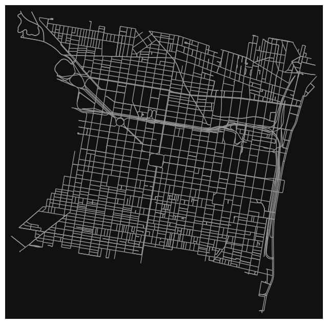

1.3 Convert your network graph edges to a GeoDataFrame

Use OSMnx to create a GeoDataFrame of the network edges in the graph object from part 1.2. The GeoDataFrame should contain the edges but not the nodes from the network.

CPD_edges = ox.graph_to_gdfs(G_CPD, edges=True, nodes=False)

CPD_edges

			osmid	oneway	name	highway	reversed	length	geometry	maxspeed	lanes	bridge	ref	tunnel	width	service	access	junction
u	v	key
109727439	109911666	0	132508434	True	Bainbridge Street	residential	False	44.137	LINESTRING (-75.17104 39.94345, -75.17053 39.9...	NaN	NaN	NaN	NaN	NaN	NaN	NaN	NaN	NaN
109727448	109727439	0	12109011	True	South Colorado Street	residential	False	109.484	LINESTRING (-75.17125 39.94248, -75.17120 39.9...	NaN	NaN	NaN	NaN	NaN	NaN	NaN	NaN	NaN
109727448	110034229	0	12159387	True	Fitzwater Street	residential	False	91.353	LINESTRING (-75.17125 39.94248, -75.17137 39.9...	NaN	NaN	NaN	NaN	NaN	NaN	NaN	NaN	NaN
109727507	110024052	0	193364514	True	Carpenter Street	residential	False	53.208	LINESTRING (-75.17196 39.93973, -75.17134 39.9...	NaN	NaN	NaN	NaN	NaN	NaN	NaN	NaN	NaN
109728761	110274344	0	672312336	True	Brown Street	residential	False	58.270	LINESTRING (-75.17317 39.96951, -75.17250 39.9...	25 mph	NaN	NaN	NaN	NaN	NaN	NaN	NaN	NaN
...	...	...	...	...	...	...	...	...	...	...	...	...	...	...	...	...	...	...
11176163640	11176163648	1	1206065012	False	NaN	living_street	False	57.963	LINESTRING (-75.16655 39.95896, -75.16633 39.9...	NaN	NaN	NaN	NaN	NaN	NaN	NaN	NaN	NaN
11176163640	5808113442	0	613950538	False	Alexander Court	living_street	True	37.086	LINESTRING (-75.16655 39.95896, -75.16662 39.9...	NaN	NaN	NaN	NaN	NaN	NaN	NaN	NaN	NaN
11176163648	5808113443	0	613950538	False	Alexander Court	living_street	False	31.592	LINESTRING (-75.16652 39.95909, -75.16646 39.9...	NaN	NaN	NaN	NaN	NaN	NaN	NaN	NaN	NaN
	11176163640	0	613950538	False	Alexander Court	living_street	True	14.738	LINESTRING (-75.16652 39.95909, -75.16655 39.9...	NaN	NaN	NaN	NaN	NaN	NaN	NaN	NaN	NaN
	11176163640	1	1206065012	False	NaN	living_street	True	57.963	LINESTRING (-75.16652 39.95909, -75.16630 39.9...	NaN	NaN	NaN	NaN	NaN	NaN	NaN	NaN	NaN

3896 rows × 16 columns

1.4 Load PennDOT crash data

Data for crashes (of all types) for 2020, 2021, and 2022 in Philadelphia County is available at the following path:

./data/CRASH_PHILADELPHIA_XXXX.csv

You should see three separate files in the data/ folder. Use pandas to read each of the CSV files, and combine them into a single dataframe using pd.concat().

The data was downloaded for Philadelphia County from here.

crash2020 = pd.read_csv("./Data/CRASH_PHILADELPHIA_2020.csv")
crash2021 = pd.read_csv("./Data/CRASH_PHILADELPHIA_2021.csv")
crash2022 = pd.read_csv("./Data/CRASH_PHILADELPHIA_2022.csv")
crashDf = pd.concat([crash2020, crash2021, crash2022])
crashDf

	CRN	ARRIVAL_TM	AUTOMOBILE_COUNT	BELTED_DEATH_COUNT	BELTED_SUSP_SERIOUS_INJ_COUNT	BICYCLE_COUNT	BICYCLE_DEATH_COUNT	BICYCLE_SUSP_SERIOUS_INJ_COUNT	BUS_COUNT	CHLDPAS_DEATH_COUNT	CHLDPAS_SUSP_SERIOUS_INJ_COUNT	COLLISION_TYPE	COMM_VEH_COUNT	CONS_ZONE_SPD_LIM	COUNTY	CRASH_MONTH	CRASH_YEAR	DAY_OF_WEEK	DEC_LAT	DEC_LONG	DISPATCH_TM	DISTRICT	DRIVER_COUNT_16YR	DRIVER_COUNT_17YR	DRIVER_COUNT_18YR	DRIVER_COUNT_19YR	DRIVER_COUNT_20YR	DRIVER_COUNT_50_64YR	DRIVER_COUNT_65_74YR	DRIVER_COUNT_75PLUS	EST_HRS_CLOSED	FATAL_COUNT	HEAVY_TRUCK_COUNT	HORSE_BUGGY_COUNT	HOUR_OF_DAY	ILLUMINATION	INJURY_COUNT	INTERSECT_TYPE	INTERSECTION_RELATED	LANE_CLOSED	LATITUDE	LN_CLOSE_DIR	LOCATION_TYPE	LONGITUDE	MAX_SEVERITY_LEVEL	MCYCLE_DEATH_COUNT	MCYCLE_SUSP_SERIOUS_INJ_COUNT	MOTORCYCLE_COUNT	MUNICIPALITY	NONMOTR_COUNT	NONMOTR_DEATH_COUNT	NONMOTR_SUSP_SERIOUS_INJ_COUNT	NTFY_HIWY_MAINT	PED_COUNT	PED_DEATH_COUNT	PED_SUSP_SERIOUS_INJ_COUNT	PERSON_COUNT	POLICE_AGCY	POSSIBLE_INJ_COUNT	RDWY_SURF_TYPE_CD	RELATION_TO_ROAD	ROAD_CONDITION	ROADWAY_CLEARED	SCH_BUS_IND	SCH_ZONE_IND	SECONDARY_CRASH	SMALL_TRUCK_COUNT	SPEC_JURIS_CD	SUSP_MINOR_INJ_COUNT	SUSP_SERIOUS_INJ_COUNT	SUV_COUNT	TCD_FUNC_CD	TCD_TYPE	TFC_DETOUR_IND	TIME_OF_DAY	TOT_INJ_COUNT	TOTAL_UNITS	UNB_DEATH_COUNT	UNB_SUSP_SERIOUS_INJ_COUNT	UNBELTED_OCC_COUNT	UNK_INJ_DEG_COUNT	UNK_INJ_PER_COUNT	URBAN_AREA	URBAN_RURAL	VAN_COUNT	VEHICLE_COUNT	WEATHER1	WEATHER2	WORK_ZONE_IND	WORK_ZONE_LOC	WORK_ZONE_TYPE	WORKERS_PRES	WZ_CLOSE_DETOUR	WZ_FLAGGER	WZ_LAW_OFFCR_IND	WZ_LN_CLOSURE	WZ_MOVING	WZ_OTHER	WZ_SHLDER_MDN	WZ_WORKERS_INJ_KILLED
0	2020036588	1349.0	1	0	0	0	0	0	0	0	0	1	0	NaN	67	3	2020	2	39.9601	-75.1794	1343.0	6	0	0	0	0	0	0	0	0	NaN	0	0	0.0	13	1	0	0	NaN	1	39 57:36.245	4.0	0	75 10:45.819	0	0	0	0	67301	0	0	0	N	0	0	0	3	68K01	0	NaN	1	9	NaN	N	N	NaN	1	NaN	0	0	0	0	0	N	1332	0	2	0	0	0	0	0	3	4	0	2	7	NaN	N	NaN	NaN	NaN	NaN	NaN	NaN	NaN	NaN	NaN	NaN	NaN
1	2020036617	1842.0	1	0	0	0	0	0	0	0	0	7	0	NaN	67	4	2020	1	39.9809	-75.2065	1840.0	6	0	0	0	0	0	0	0	0	NaN	0	0	0.0	18	1	0	0	NaN	1	39 58:51.367	3.0	0	75 12:23.366	0	0	0	0	67301	0	0	0	N	0	0	0	1	68K01	0	NaN	2	9	NaN	N	N	NaN	0	NaN	0	0	0	0	0	N	1838	0	1	0	0	0	0	0	3	4	0	1	7	7.0	N	NaN	NaN	NaN	NaN	NaN	NaN	NaN	NaN	NaN	NaN	NaN
2	2020035717	2000.0	1	0	0	0	0	0	0	0	0	2	0	NaN	67	4	2020	1	39.9269	-75.1691	2000.0	6	0	0	0	0	0	1	0	0	NaN	0	0	0.0	14	1	1	1	NaN	9	39 55:36.660	NaN	0	75 10:08.677	3	0	0	0	67301	0	0	0	N	0	0	0	2	67301	0	NaN	1	9	NaN	N	N	NaN	0	NaN	1	0	1	3	3	U	1457	1	2	0	0	0	0	0	3	4	0	2	7	4.0	N	NaN	NaN	NaN	NaN	NaN	NaN	NaN	NaN	NaN	NaN	NaN
3	2020034378	1139.0	2	0	0	0	0	0	0	0	0	1	0	NaN	67	4	2020	4	39.9237	-75.1924	1131.0	6	0	0	0	0	0	2	0	0	NaN	0	0	0.0	11	1	1	0	NaN	0	39 55:25.183	NaN	0	75 11:32.758	3	0	0	0	67301	0	0	0	N	0	0	0	3	68K01	0	NaN	1	1	NaN	N	N	NaN	1	NaN	1	0	0	0	0	NaN	1128	1	3	0	0	0	0	0	3	4	0	3	3	NaN	N	NaN	NaN	NaN	NaN	NaN	NaN	NaN	NaN	NaN	NaN	NaN
4	2020025511	345.0	1	0	0	0	0	0	0	0	0	7	0	NaN	67	3	2020	1	39.8826	-75.2450	329.0	6	0	0	0	0	0	0	0	0	NaN	0	0	0.0	3	3	2	0	NaN	0	39 52:57.717	NaN	0	75 14:41.931	3	0	0	0	67301	0	0	0	Y	0	0	0	2	68K01	0	NaN	4	1	NaN	N	N	NaN	0	NaN	2	0	0	0	0	NaN	328	2	1	0	0	0	0	0	3	4	0	1	3	3.0	N	NaN	NaN	NaN	NaN	NaN	NaN	NaN	NaN	NaN	NaN	NaN
...	...	...	...	...	...	...	...	...	...	...	...	...	...	...	...	...	...	...	...	...	...	...	...	...	...	...	...	...	...	...	...	...	...	...	...	...	...	...	...	...	...	...	...	...	...	...	...	...	...	...	...	...	...	...	...	...	...	...	...	...	...	...	...	...	...	...	...	...	...	...	...	...	...	...	...	...	...	...	...	...	...	...	...	...	...	...	...	...	...	...	...	...	...	...	...	...	...	...	...	...
8746	2022016289	2245.0	3	0	0	0	0	0	0	0	0	4	0	NaN	67	1	2022	4	40.0239	-75.1425	2242.0	6	0	0	0	1	0	0	0	0	NaN	0	0	0.0	22	3	1	1	NaN	0	40 01:25.870	NaN	0	75 08:33.165	3	0	0	0	67301	0	0	0	N	0	0	0	2	67301	0	NaN	1	1	NaN	N	N	N	0	NaN	1	0	1	3	3	NaN	2230	1	4	0	0	0	0	0	3	4	0	4	3	NaN	N	NaN	NaN	NaN	NaN	NaN	NaN	NaN	NaN	NaN	NaN	NaN
8747	2022037461	1706.0	1	0	0	0	0	0	0	0	0	7	0	NaN	67	3	2022	4	39.9583	-75.1658	1644.0	6	0	0	0	0	0	0	0	0	NaN	0	0	0.0	16	1	1	7	NaN	0	39 57:29.748	NaN	2	75 09:56.922	8	0	0	0	67301	0	0	0	N	0	0	0	2	68K01	0	NaN	2	1	NaN	N	N	N	0	NaN	0	0	0	0	0	NaN	1639	1	1	0	0	0	1	0	3	4	0	1	3	3.0	N	NaN	NaN	NaN	NaN	NaN	NaN	NaN	NaN	NaN	NaN	NaN
8748	2022014729	1721.0	1	0	0	0	0	0	0	0	0	4	0	NaN	67	1	2022	1	40.0189	-75.0495	1707.0	6	0	0	0	0	0	0	0	0	NaN	0	0	0.0	17	3	1	1	NaN	0	40 01:08.120	NaN	0	75 02:58.216	3	0	0	0	67301	0	0	0	N	0	0	0	2	67301	0	NaN	1	9	NaN	N	N	N	0	NaN	1	0	1	3	3	NaN	1701	1	2	0	0	0	0	1	3	4	0	2	3	NaN	N	NaN	NaN	NaN	NaN	NaN	NaN	NaN	NaN	NaN	NaN	NaN
8749	2022014753	713.0	3	0	0	0	0	0	0	0	0	6	0	NaN	67	2	2022	4	39.9291	-75.1687	707.0	6	0	0	0	0	0	2	0	0	NaN	0	0	0.0	7	1	2	0	N	0	39 55:44.636	NaN	0	75 10:07.421	3	0	0	0	67301	0	0	0	N	0	0	0	4	67301	0	NaN	3	1	NaN	N	N	N	1	NaN	1	0	1	0	0	NaN	700	2	5	0	0	0	1	0	3	4	0	5	5	7.0	N	NaN	NaN	NaN	NaN	NaN	NaN	NaN	NaN	NaN	NaN	NaN
8750	2022014627	1700.0	1	0	0	0	0	0	0	0	0	8	0	NaN	67	2	2022	5	39.9471	-75.1660	1646.0	6	0	0	0	0	0	0	0	0	NaN	0	0	0.0	9	1	1	0	N	0	39 56:49.690	NaN	0	75 09:57.440	3	0	0	0	67301	1	0	0	N	1	0	0	2	67301	0	NaN	1	9	NaN	N	N	N	0	NaN	1	0	0	0	0	NaN	945	1	2	0	0	0	0	0	3	4	0	1	7	7.0	N	NaN	NaN	NaN	NaN	NaN	NaN	NaN	NaN	NaN	NaN	NaN

29463 rows × 100 columns

1.5 Convert the crash data to a GeoDataFrame

You will need to use the DEC_LAT and DEC_LONG columns for latitude and longitude.

The full data dictionary for the data is available here

crashGDF = gpd.GeoDataFrame(crashDf, geometry=gpd.points_from_xy(crashDf["DEC_LONG"], crashDf["DEC_LAT"], crs="2272"))
crashGDF

	CRN	ARRIVAL_TM	AUTOMOBILE_COUNT	BELTED_DEATH_COUNT	BELTED_SUSP_SERIOUS_INJ_COUNT	BICYCLE_COUNT	BICYCLE_DEATH_COUNT	BICYCLE_SUSP_SERIOUS_INJ_COUNT	BUS_COUNT	CHLDPAS_DEATH_COUNT	CHLDPAS_SUSP_SERIOUS_INJ_COUNT	COLLISION_TYPE	COMM_VEH_COUNT	CONS_ZONE_SPD_LIM	COUNTY	CRASH_MONTH	CRASH_YEAR	DAY_OF_WEEK	DEC_LAT	DEC_LONG	DISPATCH_TM	DISTRICT	DRIVER_COUNT_16YR	DRIVER_COUNT_17YR	DRIVER_COUNT_18YR	DRIVER_COUNT_19YR	DRIVER_COUNT_20YR	DRIVER_COUNT_50_64YR	DRIVER_COUNT_65_74YR	DRIVER_COUNT_75PLUS	EST_HRS_CLOSED	FATAL_COUNT	HEAVY_TRUCK_COUNT	HORSE_BUGGY_COUNT	HOUR_OF_DAY	ILLUMINATION	INJURY_COUNT	INTERSECT_TYPE	INTERSECTION_RELATED	LANE_CLOSED	LATITUDE	LN_CLOSE_DIR	LOCATION_TYPE	LONGITUDE	MAX_SEVERITY_LEVEL	MCYCLE_DEATH_COUNT	MCYCLE_SUSP_SERIOUS_INJ_COUNT	MOTORCYCLE_COUNT	MUNICIPALITY	NONMOTR_COUNT	NONMOTR_DEATH_COUNT	NONMOTR_SUSP_SERIOUS_INJ_COUNT	NTFY_HIWY_MAINT	PED_COUNT	PED_DEATH_COUNT	PED_SUSP_SERIOUS_INJ_COUNT	PERSON_COUNT	POLICE_AGCY	POSSIBLE_INJ_COUNT	RDWY_SURF_TYPE_CD	RELATION_TO_ROAD	ROAD_CONDITION	ROADWAY_CLEARED	SCH_BUS_IND	SCH_ZONE_IND	SECONDARY_CRASH	SMALL_TRUCK_COUNT	SPEC_JURIS_CD	SUSP_MINOR_INJ_COUNT	SUSP_SERIOUS_INJ_COUNT	SUV_COUNT	TCD_FUNC_CD	TCD_TYPE	TFC_DETOUR_IND	TIME_OF_DAY	TOT_INJ_COUNT	TOTAL_UNITS	UNB_DEATH_COUNT	UNB_SUSP_SERIOUS_INJ_COUNT	UNBELTED_OCC_COUNT	UNK_INJ_DEG_COUNT	UNK_INJ_PER_COUNT	URBAN_AREA	URBAN_RURAL	VAN_COUNT	VEHICLE_COUNT	WEATHER1	WEATHER2	WORK_ZONE_IND	WORK_ZONE_LOC	WORK_ZONE_TYPE	WORKERS_PRES	WZ_CLOSE_DETOUR	WZ_FLAGGER	WZ_LAW_OFFCR_IND	WZ_LN_CLOSURE	WZ_MOVING	WZ_OTHER	WZ_SHLDER_MDN	WZ_WORKERS_INJ_KILLED	geometry
0	2020036588	1349.0	1	0	0	0	0	0	0	0	0	1	0	NaN	67	3	2020	2	39.9601	-75.1794	1343.0	6	0	0	0	0	0	0	0	0	NaN	0	0	0.0	13	1	0	0	NaN	1	39 57:36.245	4.0	0	75 10:45.819	0	0	0	0	67301	0	0	0	N	0	0	0	3	68K01	0	NaN	1	9	NaN	N	N	NaN	1	NaN	0	0	0	0	0	N	1332	0	2	0	0	0	0	0	3	4	0	2	7	NaN	N	NaN	NaN	NaN	NaN	NaN	NaN	NaN	NaN	NaN	NaN	NaN	POINT (-75.179 39.960)
1	2020036617	1842.0	1	0	0	0	0	0	0	0	0	7	0	NaN	67	4	2020	1	39.9809	-75.2065	1840.0	6	0	0	0	0	0	0	0	0	NaN	0	0	0.0	18	1	0	0	NaN	1	39 58:51.367	3.0	0	75 12:23.366	0	0	0	0	67301	0	0	0	N	0	0	0	1	68K01	0	NaN	2	9	NaN	N	N	NaN	0	NaN	0	0	0	0	0	N	1838	0	1	0	0	0	0	0	3	4	0	1	7	7.0	N	NaN	NaN	NaN	NaN	NaN	NaN	NaN	NaN	NaN	NaN	NaN	POINT (-75.207 39.981)
2	2020035717	2000.0	1	0	0	0	0	0	0	0	0	2	0	NaN	67	4	2020	1	39.9269	-75.1691	2000.0	6	0	0	0	0	0	1	0	0	NaN	0	0	0.0	14	1	1	1	NaN	9	39 55:36.660	NaN	0	75 10:08.677	3	0	0	0	67301	0	0	0	N	0	0	0	2	67301	0	NaN	1	9	NaN	N	N	NaN	0	NaN	1	0	1	3	3	U	1457	1	2	0	0	0	0	0	3	4	0	2	7	4.0	N	NaN	NaN	NaN	NaN	NaN	NaN	NaN	NaN	NaN	NaN	NaN	POINT (-75.169 39.927)
3	2020034378	1139.0	2	0	0	0	0	0	0	0	0	1	0	NaN	67	4	2020	4	39.9237	-75.1924	1131.0	6	0	0	0	0	0	2	0	0	NaN	0	0	0.0	11	1	1	0	NaN	0	39 55:25.183	NaN	0	75 11:32.758	3	0	0	0	67301	0	0	0	N	0	0	0	3	68K01	0	NaN	1	1	NaN	N	N	NaN	1	NaN	1	0	0	0	0	NaN	1128	1	3	0	0	0	0	0	3	4	0	3	3	NaN	N	NaN	NaN	NaN	NaN	NaN	NaN	NaN	NaN	NaN	NaN	NaN	POINT (-75.192 39.924)
4	2020025511	345.0	1	0	0	0	0	0	0	0	0	7	0	NaN	67	3	2020	1	39.8826	-75.2450	329.0	6	0	0	0	0	0	0	0	0	NaN	0	0	0.0	3	3	2	0	NaN	0	39 52:57.717	NaN	0	75 14:41.931	3	0	0	0	67301	0	0	0	Y	0	0	0	2	68K01	0	NaN	4	1	NaN	N	N	NaN	0	NaN	2	0	0	0	0	NaN	328	2	1	0	0	0	0	0	3	4	0	1	3	3.0	N	NaN	NaN	NaN	NaN	NaN	NaN	NaN	NaN	NaN	NaN	NaN	POINT (-75.245 39.883)
...	...	...	...	...	...	...	...	...	...	...	...	...	...	...	...	...	...	...	...	...	...	...	...	...	...	...	...	...	...	...	...	...	...	...	...	...	...	...	...	...	...	...	...	...	...	...	...	...	...	...	...	...	...	...	...	...	...	...	...	...	...	...	...	...	...	...	...	...	...	...	...	...	...	...	...	...	...	...	...	...	...	...	...	...	...	...	...	...	...	...	...	...	...	...	...	...	...	...	...	...	...
8746	2022016289	2245.0	3	0	0	0	0	0	0	0	0	4	0	NaN	67	1	2022	4	40.0239	-75.1425	2242.0	6	0	0	0	1	0	0	0	0	NaN	0	0	0.0	22	3	1	1	NaN	0	40 01:25.870	NaN	0	75 08:33.165	3	0	0	0	67301	0	0	0	N	0	0	0	2	67301	0	NaN	1	1	NaN	N	N	N	0	NaN	1	0	1	3	3	NaN	2230	1	4	0	0	0	0	0	3	4	0	4	3	NaN	N	NaN	NaN	NaN	NaN	NaN	NaN	NaN	NaN	NaN	NaN	NaN	POINT (-75.142 40.024)
8747	2022037461	1706.0	1	0	0	0	0	0	0	0	0	7	0	NaN	67	3	2022	4	39.9583	-75.1658	1644.0	6	0	0	0	0	0	0	0	0	NaN	0	0	0.0	16	1	1	7	NaN	0	39 57:29.748	NaN	2	75 09:56.922	8	0	0	0	67301	0	0	0	N	0	0	0	2	68K01	0	NaN	2	1	NaN	N	N	N	0	NaN	0	0	0	0	0	NaN	1639	1	1	0	0	0	1	0	3	4	0	1	3	3.0	N	NaN	NaN	NaN	NaN	NaN	NaN	NaN	NaN	NaN	NaN	NaN	POINT (-75.166 39.958)
8748	2022014729	1721.0	1	0	0	0	0	0	0	0	0	4	0	NaN	67	1	2022	1	40.0189	-75.0495	1707.0	6	0	0	0	0	0	0	0	0	NaN	0	0	0.0	17	3	1	1	NaN	0	40 01:08.120	NaN	0	75 02:58.216	3	0	0	0	67301	0	0	0	N	0	0	0	2	67301	0	NaN	1	9	NaN	N	N	N	0	NaN	1	0	1	3	3	NaN	1701	1	2	0	0	0	0	1	3	4	0	2	3	NaN	N	NaN	NaN	NaN	NaN	NaN	NaN	NaN	NaN	NaN	NaN	NaN	POINT (-75.049 40.019)
8749	2022014753	713.0	3	0	0	0	0	0	0	0	0	6	0	NaN	67	2	2022	4	39.9291	-75.1687	707.0	6	0	0	0	0	0	2	0	0	NaN	0	0	0.0	7	1	2	0	N	0	39 55:44.636	NaN	0	75 10:07.421	3	0	0	0	67301	0	0	0	N	0	0	0	4	67301	0	NaN	3	1	NaN	N	N	N	1	NaN	1	0	1	0	0	NaN	700	2	5	0	0	0	1	0	3	4	0	5	5	7.0	N	NaN	NaN	NaN	NaN	NaN	NaN	NaN	NaN	NaN	NaN	NaN	POINT (-75.169 39.929)
8750	2022014627	1700.0	1	0	0	0	0	0	0	0	0	8	0	NaN	67	2	2022	5	39.9471	-75.1660	1646.0	6	0	0	0	0	0	0	0	0	NaN	0	0	0.0	9	1	1	0	N	0	39 56:49.690	NaN	0	75 09:57.440	3	0	0	0	67301	1	0	0	N	1	0	0	2	67301	0	NaN	1	9	NaN	N	N	N	0	NaN	1	0	0	0	0	NaN	945	1	2	0	0	0	0	0	3	4	0	1	7	7.0	N	NaN	NaN	NaN	NaN	NaN	NaN	NaN	NaN	NaN	NaN	NaN	POINT (-75.166 39.947)

29463 rows × 101 columns

1.6 Trim the crash data to Center City

Get the boundary of the edges data frame (from part 1.3). Accessing the .geometry.unary_union.convex_hull property will give you a nice outer boundary region.
Trim the crashes using the within() function of the crash GeoDataFrame to find which crashes are within the boundary.

There should be about 3,750 crashes within the Central district.

CPD_boundary = CPD_edges.geometry.unary_union.convex_hull
CC_crashes = crashGDF[crashGDF.within(CPD_boundary)]
CC_crashes

	CRN	ARRIVAL_TM	AUTOMOBILE_COUNT	BELTED_DEATH_COUNT	BELTED_SUSP_SERIOUS_INJ_COUNT	BICYCLE_COUNT	BICYCLE_DEATH_COUNT	BICYCLE_SUSP_SERIOUS_INJ_COUNT	BUS_COUNT	CHLDPAS_DEATH_COUNT	CHLDPAS_SUSP_SERIOUS_INJ_COUNT	COLLISION_TYPE	COMM_VEH_COUNT	CONS_ZONE_SPD_LIM	COUNTY	CRASH_MONTH	CRASH_YEAR	DAY_OF_WEEK	DEC_LAT	DEC_LONG	DISPATCH_TM	DISTRICT	DRIVER_COUNT_16YR	DRIVER_COUNT_17YR	DRIVER_COUNT_18YR	DRIVER_COUNT_19YR	DRIVER_COUNT_20YR	DRIVER_COUNT_50_64YR	DRIVER_COUNT_65_74YR	DRIVER_COUNT_75PLUS	EST_HRS_CLOSED	FATAL_COUNT	HEAVY_TRUCK_COUNT	HORSE_BUGGY_COUNT	HOUR_OF_DAY	ILLUMINATION	INJURY_COUNT	INTERSECT_TYPE	INTERSECTION_RELATED	LANE_CLOSED	LATITUDE	LN_CLOSE_DIR	LOCATION_TYPE	LONGITUDE	MAX_SEVERITY_LEVEL	MCYCLE_DEATH_COUNT	MCYCLE_SUSP_SERIOUS_INJ_COUNT	MOTORCYCLE_COUNT	MUNICIPALITY	NONMOTR_COUNT	NONMOTR_DEATH_COUNT	NONMOTR_SUSP_SERIOUS_INJ_COUNT	NTFY_HIWY_MAINT	PED_COUNT	PED_DEATH_COUNT	PED_SUSP_SERIOUS_INJ_COUNT	PERSON_COUNT	POLICE_AGCY	POSSIBLE_INJ_COUNT	RDWY_SURF_TYPE_CD	RELATION_TO_ROAD	ROAD_CONDITION	ROADWAY_CLEARED	SCH_BUS_IND	SCH_ZONE_IND	SECONDARY_CRASH	SMALL_TRUCK_COUNT	SPEC_JURIS_CD	SUSP_MINOR_INJ_COUNT	SUSP_SERIOUS_INJ_COUNT	SUV_COUNT	TCD_FUNC_CD	TCD_TYPE	TFC_DETOUR_IND	TIME_OF_DAY	TOT_INJ_COUNT	TOTAL_UNITS	UNB_DEATH_COUNT	UNB_SUSP_SERIOUS_INJ_COUNT	UNBELTED_OCC_COUNT	UNK_INJ_DEG_COUNT	UNK_INJ_PER_COUNT	URBAN_AREA	URBAN_RURAL	VAN_COUNT	VEHICLE_COUNT	WEATHER1	WEATHER2	WORK_ZONE_IND	WORK_ZONE_LOC	WORK_ZONE_TYPE	WORKERS_PRES	WZ_CLOSE_DETOUR	WZ_FLAGGER	WZ_LAW_OFFCR_IND	WZ_LN_CLOSURE	WZ_MOVING	WZ_OTHER	WZ_SHLDER_MDN	WZ_WORKERS_INJ_KILLED	geometry
0	2020036588	1349.0	1	0	0	0	0	0	0	0	0	1	0	NaN	67	3	2020	2	39.9601	-75.1794	1343.0	6	0	0	0	0	0	0	0	0	NaN	0	0	0.0	13	1	0	0	NaN	1	39 57:36.245	4.0	0	75 10:45.819	0	0	0	0	67301	0	0	0	N	0	0	0	3	68K01	0	NaN	1	9	NaN	N	N	NaN	1	NaN	0	0	0	0	0	N	1332	0	2	0	0	0	0	0	3	4	0	2	7	NaN	N	NaN	NaN	NaN	NaN	NaN	NaN	NaN	NaN	NaN	NaN	NaN	POINT (-75.179 39.960)
7	2020035021	1255.0	1	0	0	0	0	0	1	0	0	4	1	NaN	67	3	2020	2	39.9700	-75.1631	1250.0	6	0	0	0	0	0	1	0	0	NaN	0	0	0.0	12	1	2	1	NaN	0	39 58:11.995	NaN	0	75 09:47.193	8	0	0	0	67301	0	0	0	N	0	0	0	4	67508	0	NaN	1	1	NaN	N	N	NaN	0	NaN	0	0	0	3	3	N	1250	2	2	0	0	0	2	1	3	4	0	2	3	NaN	N	NaN	NaN	NaN	NaN	NaN	NaN	NaN	NaN	NaN	NaN	NaN	POINT (-75.163 39.970)
11	2020021944	805.0	2	0	0	0	0	0	0	0	0	1	0	NaN	67	2	2020	7	39.9523	-75.1878	800.0	6	0	0	0	0	0	0	0	0	NaN	0	0	0.0	8	1	2	0	NaN	2	39 57:08.258	4.0	0	75 11:16.213	3	0	0	0	67301	0	0	0	N	0	0	0	2	67504	0	NaN	6	1	NaN	N	N	NaN	0	NaN	2	0	0	0	0	N	800	2	2	0	0	2	0	0	3	4	0	2	3	3.0	N	NaN	NaN	NaN	NaN	NaN	NaN	NaN	NaN	NaN	NaN	NaN	POINT (-75.188 39.952)
12	2020024963	1024.0	1	0	0	0	0	0	0	0	0	5	1	NaN	67	3	2020	2	39.9558	-75.1484	1024.0	6	0	0	0	0	0	0	0	0	NaN	0	1	0.0	10	1	0	0	NaN	0	39 57:21.042	NaN	2	75 08:54.233	0	0	0	0	67301	0	0	0	N	0	0	0	2	67501	0	NaN	1	1	NaN	N	N	NaN	0	NaN	0	0	0	0	0	NaN	1024	0	2	0	0	0	0	0	3	4	0	2	3	3.0	N	NaN	NaN	NaN	NaN	NaN	NaN	NaN	NaN	NaN	NaN	NaN	POINT (-75.148 39.956)
18	2020000481	1737.0	1	0	0	0	0	0	1	0	0	5	1	NaN	67	1	2020	4	39.9534	-75.1547	1737.0	6	0	0	0	0	0	0	0	0	NaN	0	0	0.0	17	4	0	1	NaN	0	39 57:12.069	NaN	0	75 09:16.934	0	0	0	0	67301	0	0	0	N	0	0	0	2	67301	0	NaN	1	1	NaN	N	N	NaN	0	NaN	0	0	0	3	2	NaN	1735	0	2	0	0	0	0	0	3	4	0	2	3	NaN	N	NaN	NaN	NaN	NaN	NaN	NaN	NaN	NaN	NaN	NaN	NaN	POINT (-75.155 39.953)
...	...	...	...	...	...	...	...	...	...	...	...	...	...	...	...	...	...	...	...	...	...	...	...	...	...	...	...	...	...	...	...	...	...	...	...	...	...	...	...	...	...	...	...	...	...	...	...	...	...	...	...	...	...	...	...	...	...	...	...	...	...	...	...	...	...	...	...	...	...	...	...	...	...	...	...	...	...	...	...	...	...	...	...	...	...	...	...	...	...	...	...	...	...	...	...	...	...	...	...	...	...
8719	2022019573	2210.0	0	0	0	0	0	0	0	0	0	8	0	NaN	67	1	2022	5	39.9556	-75.1728	2205.0	6	0	0	0	0	0	0	0	0	NaN	0	0	0.0	21	3	1	1	NaN	0	39 57:20.163	NaN	0	75 10:21.961	3	0	0	0	67301	1	0	0	N	1	0	0	2	67301	0	NaN	1	1	NaN	N	N	N	0	NaN	1	0	1	3	2	NaN	2145	1	2	0	0	0	0	1	3	4	0	1	3	3.0	N	NaN	NaN	NaN	NaN	NaN	NaN	NaN	NaN	NaN	NaN	NaN	POINT (-75.173 39.956)
8723	2022037448	252.0	1	0	0	0	0	0	0	0	0	7	0	NaN	67	2	2022	1	39.9537	-75.1816	237.0	6	0	0	0	0	0	1	0	0	NaN	0	0	0.0	2	3	1	0	N	1	39 57:13.320	3.0	0	75 10:53.702	4	0	0	0	67301	0	0	0	N	0	0	0	1	68K01	1	NaN	2	1	246.0	N	N	N	0	NaN	0	0	0	0	0	N	236	1	1	0	0	0	0	0	3	4	0	1	3	NaN	N	NaN	NaN	NaN	NaN	NaN	NaN	NaN	NaN	NaN	NaN	NaN	POINT (-75.182 39.954)
8744	2022037464	2225.0	1	0	0	0	0	0	0	0	0	1	0	NaN	67	3	2022	5	39.9600	-75.1798	2210.0	6	0	0	0	0	0	0	0	0	NaN	0	0	0.0	22	3	0	6	NaN	0	39 57:36.017	NaN	2	75 10:47.219	0	0	0	0	67301	0	0	0	N	0	0	0	2	68K01	0	NaN	1	9	NaN	N	N	N	0	NaN	0	0	1	0	0	NaN	2205	0	2	0	0	0	0	0	3	4	0	2	7	7.0	N	NaN	NaN	NaN	NaN	NaN	NaN	NaN	NaN	NaN	NaN	NaN	POINT (-75.180 39.960)
8747	2022037461	1706.0	1	0	0	0	0	0	0	0	0	7	0	NaN	67	3	2022	4	39.9583	-75.1658	1644.0	6	0	0	0	0	0	0	0	0	NaN	0	0	0.0	16	1	1	7	NaN	0	39 57:29.748	NaN	2	75 09:56.922	8	0	0	0	67301	0	0	0	N	0	0	0	2	68K01	0	NaN	2	1	NaN	N	N	N	0	NaN	0	0	0	0	0	NaN	1639	1	1	0	0	0	1	0	3	4	0	1	3	3.0	N	NaN	NaN	NaN	NaN	NaN	NaN	NaN	NaN	NaN	NaN	NaN	POINT (-75.166 39.958)
8750	2022014627	1700.0	1	0	0	0	0	0	0	0	0	8	0	NaN	67	2	2022	5	39.9471	-75.1660	1646.0	6	0	0	0	0	0	0	0	0	NaN	0	0	0.0	9	1	1	0	N	0	39 56:49.690	NaN	0	75 09:57.440	3	0	0	0	67301	1	0	0	N	1	0	0	2	67301	0	NaN	1	9	NaN	N	N	N	0	NaN	1	0	0	0	0	NaN	945	1	2	0	0	0	0	0	3	4	0	1	7	7.0	N	NaN	NaN	NaN	NaN	NaN	NaN	NaN	NaN	NaN	NaN	NaN	POINT (-75.166 39.947)

3751 rows × 101 columns

1.7 Re-project our data into an approriate CRS

We’ll need to find the nearest edge (street) in our graph for each crash. To do this, osmnx will calculate the distance from each crash to the graph edges. For this calculation to be accurate, we need to convert from latitude/longitude

We’ll convert the local state plane CRS for Philadelphia, EPSG=2272

Two steps:

Project the graph object (G) using the ox.project_graph. Run ox.project_graph? to see the documentation for how to convert to a specific CRS.
Project the crash data using the .to_crs() function.

G_projected = ox.project_graph(G_CPD, to_crs=2272)
CC_crashproj = CC_crashes.to_crs(2272)
CC_crashproj

	CRN	ARRIVAL_TM	AUTOMOBILE_COUNT	BELTED_DEATH_COUNT	BELTED_SUSP_SERIOUS_INJ_COUNT	BICYCLE_COUNT	BICYCLE_DEATH_COUNT	BICYCLE_SUSP_SERIOUS_INJ_COUNT	BUS_COUNT	CHLDPAS_DEATH_COUNT	CHLDPAS_SUSP_SERIOUS_INJ_COUNT	COLLISION_TYPE	COMM_VEH_COUNT	CONS_ZONE_SPD_LIM	COUNTY	CRASH_MONTH	CRASH_YEAR	DAY_OF_WEEK	DEC_LAT	DEC_LONG	DISPATCH_TM	DISTRICT	DRIVER_COUNT_16YR	DRIVER_COUNT_17YR	DRIVER_COUNT_18YR	DRIVER_COUNT_19YR	DRIVER_COUNT_20YR	DRIVER_COUNT_50_64YR	DRIVER_COUNT_65_74YR	DRIVER_COUNT_75PLUS	EST_HRS_CLOSED	FATAL_COUNT	HEAVY_TRUCK_COUNT	HORSE_BUGGY_COUNT	HOUR_OF_DAY	ILLUMINATION	INJURY_COUNT	INTERSECT_TYPE	INTERSECTION_RELATED	LANE_CLOSED	LATITUDE	LN_CLOSE_DIR	LOCATION_TYPE	LONGITUDE	MAX_SEVERITY_LEVEL	MCYCLE_DEATH_COUNT	MCYCLE_SUSP_SERIOUS_INJ_COUNT	MOTORCYCLE_COUNT	MUNICIPALITY	NONMOTR_COUNT	NONMOTR_DEATH_COUNT	NONMOTR_SUSP_SERIOUS_INJ_COUNT	NTFY_HIWY_MAINT	PED_COUNT	PED_DEATH_COUNT	PED_SUSP_SERIOUS_INJ_COUNT	PERSON_COUNT	POLICE_AGCY	POSSIBLE_INJ_COUNT	RDWY_SURF_TYPE_CD	RELATION_TO_ROAD	ROAD_CONDITION	ROADWAY_CLEARED	SCH_BUS_IND	SCH_ZONE_IND	SECONDARY_CRASH	SMALL_TRUCK_COUNT	SPEC_JURIS_CD	SUSP_MINOR_INJ_COUNT	SUSP_SERIOUS_INJ_COUNT	SUV_COUNT	TCD_FUNC_CD	TCD_TYPE	TFC_DETOUR_IND	TIME_OF_DAY	TOT_INJ_COUNT	TOTAL_UNITS	UNB_DEATH_COUNT	UNB_SUSP_SERIOUS_INJ_COUNT	UNBELTED_OCC_COUNT	UNK_INJ_DEG_COUNT	UNK_INJ_PER_COUNT	URBAN_AREA	URBAN_RURAL	VAN_COUNT	VEHICLE_COUNT	WEATHER1	WEATHER2	WORK_ZONE_IND	WORK_ZONE_LOC	WORK_ZONE_TYPE	WORKERS_PRES	WZ_CLOSE_DETOUR	WZ_FLAGGER	WZ_LAW_OFFCR_IND	WZ_LN_CLOSURE	WZ_MOVING	WZ_OTHER	WZ_SHLDER_MDN	WZ_WORKERS_INJ_KILLED	geometry
0	2020036588	1349.0	1	0	0	0	0	0	0	0	0	1	0	NaN	67	3	2020	2	39.9601	-75.1794	1343.0	6	0	0	0	0	0	0	0	0	NaN	0	0	0.0	13	1	0	0	NaN	1	39 57:36.245	4.0	0	75 10:45.819	0	0	0	0	67301	0	0	0	N	0	0	0	3	68K01	0	NaN	1	9	NaN	N	N	NaN	1	NaN	0	0	0	0	0	N	1332	0	2	0	0	0	0	0	3	4	0	2	7	NaN	N	NaN	NaN	NaN	NaN	NaN	NaN	NaN	NaN	NaN	NaN	NaN	POINT (-75.179 39.960)
7	2020035021	1255.0	1	0	0	0	0	0	1	0	0	4	1	NaN	67	3	2020	2	39.9700	-75.1631	1250.0	6	0	0	0	0	0	1	0	0	NaN	0	0	0.0	12	1	2	1	NaN	0	39 58:11.995	NaN	0	75 09:47.193	8	0	0	0	67301	0	0	0	N	0	0	0	4	67508	0	NaN	1	1	NaN	N	N	NaN	0	NaN	0	0	0	3	3	N	1250	2	2	0	0	0	2	1	3	4	0	2	3	NaN	N	NaN	NaN	NaN	NaN	NaN	NaN	NaN	NaN	NaN	NaN	NaN	POINT (-75.163 39.970)
11	2020021944	805.0	2	0	0	0	0	0	0	0	0	1	0	NaN	67	2	2020	7	39.9523	-75.1878	800.0	6	0	0	0	0	0	0	0	0	NaN	0	0	0.0	8	1	2	0	NaN	2	39 57:08.258	4.0	0	75 11:16.213	3	0	0	0	67301	0	0	0	N	0	0	0	2	67504	0	NaN	6	1	NaN	N	N	NaN	0	NaN	2	0	0	0	0	N	800	2	2	0	0	2	0	0	3	4	0	2	3	3.0	N	NaN	NaN	NaN	NaN	NaN	NaN	NaN	NaN	NaN	NaN	NaN	POINT (-75.188 39.952)
12	2020024963	1024.0	1	0	0	0	0	0	0	0	0	5	1	NaN	67	3	2020	2	39.9558	-75.1484	1024.0	6	0	0	0	0	0	0	0	0	NaN	0	1	0.0	10	1	0	0	NaN	0	39 57:21.042	NaN	2	75 08:54.233	0	0	0	0	67301	0	0	0	N	0	0	0	2	67501	0	NaN	1	1	NaN	N	N	NaN	0	NaN	0	0	0	0	0	NaN	1024	0	2	0	0	0	0	0	3	4	0	2	3	3.0	N	NaN	NaN	NaN	NaN	NaN	NaN	NaN	NaN	NaN	NaN	NaN	POINT (-75.148 39.956)
18	2020000481	1737.0	1	0	0	0	0	0	1	0	0	5	1	NaN	67	1	2020	4	39.9534	-75.1547	1737.0	6	0	0	0	0	0	0	0	0	NaN	0	0	0.0	17	4	0	1	NaN	0	39 57:12.069	NaN	0	75 09:16.934	0	0	0	0	67301	0	0	0	N	0	0	0	2	67301	0	NaN	1	1	NaN	N	N	NaN	0	NaN	0	0	0	3	2	NaN	1735	0	2	0	0	0	0	0	3	4	0	2	3	NaN	N	NaN	NaN	NaN	NaN	NaN	NaN	NaN	NaN	NaN	NaN	NaN	POINT (-75.155 39.953)
...	...	...	...	...	...	...	...	...	...	...	...	...	...	...	...	...	...	...	...	...	...	...	...	...	...	...	...	...	...	...	...	...	...	...	...	...	...	...	...	...	...	...	...	...	...	...	...	...	...	...	...	...	...	...	...	...	...	...	...	...	...	...	...	...	...	...	...	...	...	...	...	...	...	...	...	...	...	...	...	...	...	...	...	...	...	...	...	...	...	...	...	...	...	...	...	...	...	...	...	...	...
8719	2022019573	2210.0	0	0	0	0	0	0	0	0	0	8	0	NaN	67	1	2022	5	39.9556	-75.1728	2205.0	6	0	0	0	0	0	0	0	0	NaN	0	0	0.0	21	3	1	1	NaN	0	39 57:20.163	NaN	0	75 10:21.961	3	0	0	0	67301	1	0	0	N	1	0	0	2	67301	0	NaN	1	1	NaN	N	N	N	0	NaN	1	0	1	3	2	NaN	2145	1	2	0	0	0	0	1	3	4	0	1	3	3.0	N	NaN	NaN	NaN	NaN	NaN	NaN	NaN	NaN	NaN	NaN	NaN	POINT (-75.173 39.956)
8723	2022037448	252.0	1	0	0	0	0	0	0	0	0	7	0	NaN	67	2	2022	1	39.9537	-75.1816	237.0	6	0	0	0	0	0	1	0	0	NaN	0	0	0.0	2	3	1	0	N	1	39 57:13.320	3.0	0	75 10:53.702	4	0	0	0	67301	0	0	0	N	0	0	0	1	68K01	1	NaN	2	1	246.0	N	N	N	0	NaN	0	0	0	0	0	N	236	1	1	0	0	0	0	0	3	4	0	1	3	NaN	N	NaN	NaN	NaN	NaN	NaN	NaN	NaN	NaN	NaN	NaN	NaN	POINT (-75.182 39.954)
8744	2022037464	2225.0	1	0	0	0	0	0	0	0	0	1	0	NaN	67	3	2022	5	39.9600	-75.1798	2210.0	6	0	0	0	0	0	0	0	0	NaN	0	0	0.0	22	3	0	6	NaN	0	39 57:36.017	NaN	2	75 10:47.219	0	0	0	0	67301	0	0	0	N	0	0	0	2	68K01	0	NaN	1	9	NaN	N	N	N	0	NaN	0	0	1	0	0	NaN	2205	0	2	0	0	0	0	0	3	4	0	2	7	7.0	N	NaN	NaN	NaN	NaN	NaN	NaN	NaN	NaN	NaN	NaN	NaN	POINT (-75.180 39.960)
8747	2022037461	1706.0	1	0	0	0	0	0	0	0	0	7	0	NaN	67	3	2022	4	39.9583	-75.1658	1644.0	6	0	0	0	0	0	0	0	0	NaN	0	0	0.0	16	1	1	7	NaN	0	39 57:29.748	NaN	2	75 09:56.922	8	0	0	0	67301	0	0	0	N	0	0	0	2	68K01	0	NaN	2	1	NaN	N	N	N	0	NaN	0	0	0	0	0	NaN	1639	1	1	0	0	0	1	0	3	4	0	1	3	3.0	N	NaN	NaN	NaN	NaN	NaN	NaN	NaN	NaN	NaN	NaN	NaN	POINT (-75.166 39.958)
8750	2022014627	1700.0	1	0	0	0	0	0	0	0	0	8	0	NaN	67	2	2022	5	39.9471	-75.1660	1646.0	6	0	0	0	0	0	0	0	0	NaN	0	0	0.0	9	1	1	0	N	0	39 56:49.690	NaN	0	75 09:57.440	3	0	0	0	67301	1	0	0	N	1	0	0	2	67301	0	NaN	1	9	NaN	N	N	N	0	NaN	1	0	0	0	0	NaN	945	1	2	0	0	0	0	0	3	4	0	1	7	7.0	N	NaN	NaN	NaN	NaN	NaN	NaN	NaN	NaN	NaN	NaN	NaN	POINT (-75.166 39.947)

3751 rows × 101 columns

ox.plot_graph(G_projected);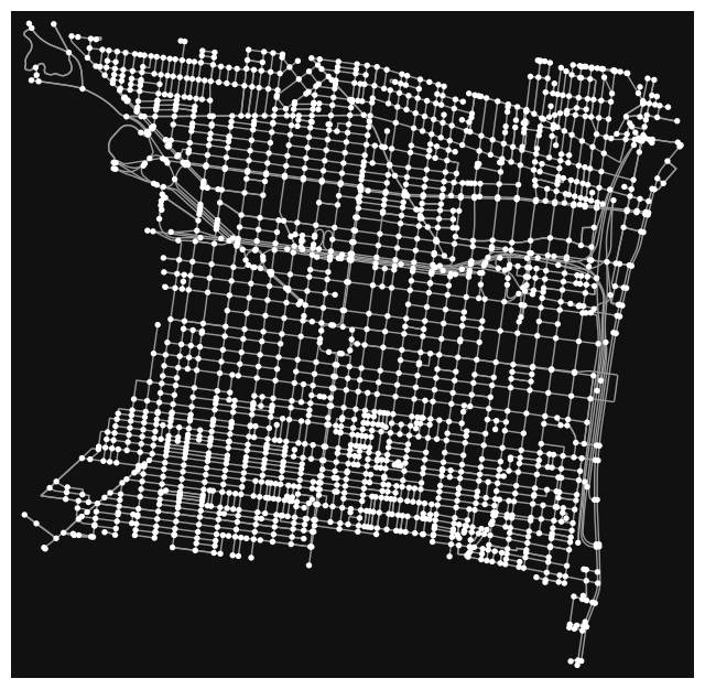

1.8 Find the nearest edge for each crash

See: ox.distance.nearest_edges(). It takes three arguments:

the network graph
the longitude of your crash data (the x attribute of the geometry column)
the latitude of your crash data (the y attribute of the geometry column)

You will get a numpy array with 3 columns that represent (u, v, key) where each u and v are the node IDs that the edge links together. We will ignore the key value for our analysis.

def find_nearest_edge(CC_crashproj, G_CPD):
    crash_longitudes = CC_crashproj.geometry.x
    crash_latitudes = CC_crashproj.geometry.y

    nearest_edges = ox.distance.nearest_edges(G_CPD, crash_longitudes, crash_latitudes)
    #CC_crashproj["nearest_edge"] = nearest_edges
    return nearest_edges

crashes_nearest_edge = find_nearest_edge(CC_crashproj, G_CPD)
#crashes_nearest_edge

1.9 Calculate the total number of crashes per street

Make a DataFrame from your data from part 1.7 with three columns, u, v, and key (we will only use the u and v columns)
Group by u and v and calculate the size
Reset the index and name your size() column as crash_count

After this step you should have a DataFrame with three columns: u, v, and crash_count.

CC_crashproj.head(4)

	CRN	ARRIVAL_TM	AUTOMOBILE_COUNT	BUS_COUNT	COLLISION_TYPE	COMM_VEH_COUNT	CONS_ZONE_SPD_LIM	COUNTY	CRASH_MONTH	CRASH_YEAR	DAY_OF_WEEK	DEC_LAT	DEC_LONG	DISPATCH_TM	DISTRICT	DRIVER_COUNT_50_64YR	EST_HRS_CLOSED	HEAVY_TRUCK_COUNT	HOUR_OF_DAY	ILLUMINATION	INJURY_COUNT	INTERSECT_TYPE	INTERSECTION_RELATED	LANE_CLOSED	LATITUDE	LN_CLOSE_DIR	LOCATION_TYPE	LONGITUDE	MAX_SEVERITY_LEVEL	MUNICIPALITY	NTFY_HIWY_MAINT	PERSON_COUNT	POLICE_AGCY	RDWY_SURF_TYPE_CD	RELATION_TO_ROAD	ROAD_CONDITION	ROADWAY_CLEARED	SCH_BUS_IND	SCH_ZONE_IND	SECONDARY_CRASH	SMALL_TRUCK_COUNT	SPEC_JURIS_CD	SUSP_MINOR_INJ_COUNT	TCD_FUNC_CD	TCD_TYPE	TFC_DETOUR_IND	TIME_OF_DAY	TOT_INJ_COUNT	TOTAL_UNITS	UNBELTED_OCC_COUNT	UNK_INJ_DEG_COUNT	UNK_INJ_PER_COUNT	URBAN_AREA	URBAN_RURAL	VEHICLE_COUNT	WEATHER1	WEATHER2	WORK_ZONE_IND	WORK_ZONE_LOC	WORK_ZONE_TYPE	WORKERS_PRES	WZ_CLOSE_DETOUR	WZ_FLAGGER	WZ_LAW_OFFCR_IND	WZ_LN_CLOSURE	WZ_MOVING	WZ_OTHER	WZ_SHLDER_MDN	WZ_WORKERS_INJ_KILLED	geometry
0	2020036588	1349.0	1	0	1	0	NaN	67	3	2020	2	39.9601	-75.1794	1343.0	6	0	NaN	0	13	1	0	0	NaN	1	39 57:36.245	4.0	0	75 10:45.819	0	67301	N	3	68K01	NaN	1	9	NaN	N	N	NaN	1	NaN	0	0	0	N	1332	0	2	0	0	0	3	4	2	7	NaN	N	NaN	NaN	NaN	NaN	NaN	NaN	NaN	NaN	NaN	NaN	NaN	POINT (-75.179 39.960)
7	2020035021	1255.0	1	1	4	1	NaN	67	3	2020	2	39.9700	-75.1631	1250.0	6	1	NaN	0	12	1	2	1	NaN	0	39 58:11.995	NaN	0	75 09:47.193	8	67301	N	4	67508	NaN	1	1	NaN	N	N	NaN	0	NaN	0	3	3	N	1250	2	2	0	2	1	3	4	2	3	NaN	N	NaN	NaN	NaN	NaN	NaN	NaN	NaN	NaN	NaN	NaN	NaN	POINT (-75.163 39.970)
11	2020021944	805.0	2	0	1	0	NaN	67	2	2020	7	39.9523	-75.1878	800.0	6	0	NaN	0	8	1	2	0	NaN	2	39 57:08.258	4.0	0	75 11:16.213	3	67301	N	2	67504	NaN	6	1	NaN	N	N	NaN	0	NaN	2	0	0	N	800	2	2	2	0	0	3	4	2	3	3.0	N	NaN	NaN	NaN	NaN	NaN	NaN	NaN	NaN	NaN	NaN	NaN	POINT (-75.188 39.952)
12	2020024963	1024.0	1	0	5	1	NaN	67	3	2020	2	39.9558	-75.1484	1024.0	6	0	NaN	1	10	1	0	0	NaN	0	39 57:21.042	NaN	2	75 08:54.233	0	67301	N	2	67501	NaN	1	1	NaN	N	N	NaN	0	NaN	0	0	0	NaN	1024	0	2	0	0	0	3	4	2	3	3.0	N	NaN	NaN	NaN	NaN	NaN	NaN	NaN	NaN	NaN	NaN	NaN	POINT (-75.148 39.956)

nearest_edge_column = crashes_nearest_edge

NearestEdgedf = pd.DataFrame(nearest_edge_column, columns=["u", "v", "key"])

NearestEdgedf

	u	v	key
0	8482829382	7065714513	0
1	109848091	109848089	0
2	1903608761	109775193	0
3	775424610	775424581	0
4	110416511	110417392	0
...	...	...	...
3746	110053344	110053369	0
3747	110453046	110318202	0
3748	8482829382	7065714513	0
3749	109791270	109783164	0
3750	110338911	110000903	0

3751 rows × 3 columns

grouped_NearestEdgedf = NearestEdgedf.groupby(["u", "v"])


crash_count = grouped_NearestEdgedf.size().to_frame('size')
crash_count_df = crash_count.reset_index()
crash_count_df.rename(columns={"size": "crash_count"}, inplace=True)
crash_count_df

	u	v	crash_count
0	109729474	3425014859	2
1	109729486	110342146	4
2	109729673	109729699	3
3	109729699	109811674	6
4	109729709	109729731	3
...	...	...	...
875	10270051289	5519334546	5
876	10660521817	10660521823	1
877	10674041689	10674041689	22
878	11144117753	109729699	3
879	11162290432	110329835	1

880 rows × 3 columns

1.10 Merge your edges GeoDataFrame and crash count DataFrame

You can use pandas to merge them on the u and v columns. This will associate the total crash count with each edge in the street network.

Tips: - Use a left merge where the first argument of the merge is the edges GeoDataFrame. This ensures no edges are removed during the merge. - Use the fillna(0) function to fill in missing crash count values with zero.

merged_CPD = pd.merge(CPD_edges, crash_count_df, how="left", on=["u","v"]).fillna(0)
merged_CPD

	u	v	osmid	oneway	name	highway	reversed	length	geometry	maxspeed	lanes	bridge	ref	tunnel	width	service	access	junction	crash_count
0	109727439	109911666	132508434	True	Bainbridge Street	residential	False	44.137	LINESTRING (-75.17104 39.94345, -75.17053 39.9...	0	0	0	0	0	0	0	0	0	0.0
1	109727448	109727439	12109011	True	South Colorado Street	residential	False	109.484	LINESTRING (-75.17125 39.94248, -75.17120 39.9...	0	0	0	0	0	0	0	0	0	0.0
2	109727448	110034229	12159387	True	Fitzwater Street	residential	False	91.353	LINESTRING (-75.17125 39.94248, -75.17137 39.9...	0	0	0	0	0	0	0	0	0	0.0
3	109727507	110024052	193364514	True	Carpenter Street	residential	False	53.208	LINESTRING (-75.17196 39.93973, -75.17134 39.9...	0	0	0	0	0	0	0	0	0	0.0
4	109728761	110274344	672312336	True	Brown Street	residential	False	58.270	LINESTRING (-75.17317 39.96951, -75.17250 39.9...	25 mph	0	0	0	0	0	0	0	0	0.0
...	...	...	...	...	...	...	...	...	...	...	...	...	...	...	...	...	...	...	...
3891	11176163640	11176163648	1206065012	False	0	living_street	False	57.963	LINESTRING (-75.16655 39.95896, -75.16633 39.9...	0	0	0	0	0	0	0	0	0	0.0
3892	11176163640	5808113442	613950538	False	Alexander Court	living_street	True	37.086	LINESTRING (-75.16655 39.95896, -75.16662 39.9...	0	0	0	0	0	0	0	0	0	0.0
3893	11176163648	5808113443	613950538	False	Alexander Court	living_street	False	31.592	LINESTRING (-75.16652 39.95909, -75.16646 39.9...	0	0	0	0	0	0	0	0	0	0.0
3894	11176163648	11176163640	613950538	False	Alexander Court	living_street	True	14.738	LINESTRING (-75.16652 39.95909, -75.16655 39.9...	0	0	0	0	0	0	0	0	0	0.0
3895	11176163648	11176163640	1206065012	False	0	living_street	True	57.963	LINESTRING (-75.16652 39.95909, -75.16630 39.9...	0	0	0	0	0	0	0	0	0	0.0

3896 rows × 19 columns

1.11 Calculate a “Crash Index”

Let’s calculate a “crash index” that provides a normalized measure of the crash frequency per street. To do this, we’ll need to:

Calculate the total crash count divided by the street length, using the length column
Perform a log transformation of the crash/length variable — use numpy’s log10() function
Normalize the index from 0 to 1 (see the lecture notes for an example of this transformation)

Note: since the crash index involves a log transformation, you should only calculate the index for streets where the crash count is greater than zero.

After this step, you should have a new column in the data frame from 1.9 that includes a column called part 1.9.

merged_CPD['crash_count_real']= merged_CPD['crash_count'].where(merged_CPD['crash_count'] > 0)
merged_CPD = merged_CPD.dropna(axis=0)

merged_CPD["crash_per_length"] = merged_CPD['crash_count'] / merged_CPD["length"]
merged_CPD["crash_index"] = np.log10(merged_CPD["crash_per_length"]) 
crash_index = merged_CPD["crash_index"]
merged_CPD["crash_index_normalized"] = (crash_index - crash_index.min()) / (crash_index.max() - crash_index.min())
merged_CPD

C:\Users\Owner\miniforge3\envs\musa-550-fall-2023\lib\site-packages\geopandas\geodataframe.py:1538: SettingWithCopyWarning: 
A value is trying to be set on a copy of a slice from a DataFrame.
Try using .loc[row_indexer,col_indexer] = value instead

See the caveats in the documentation: https://pandas.pydata.org/pandas-docs/stable/user_guide/indexing.html#returning-a-view-versus-a-copy
  super().__setitem__(key, value)

	u	v	osmid	oneway	name	highway	reversed	length	geometry	maxspeed	lanes	bridge	ref	tunnel	width	service	access	junction	crash_count	crash_count_real	crash_per_length	crash_index	crash_index_normalized
14	109729474	3425014859	62154356	True	Arch Street	secondary	False	126.087	LINESTRING (-75.14847 39.95259, -75.14859 39.9...	25 mph	2	0	0	0	0	0	0	0	2.0	2.0	0.015862	-1.799640	0.253014
15	109729486	110342146	[12169305, 1052694387]	True	North Independence Mall East	secondary	False	123.116	LINESTRING (-75.14832 39.95333, -75.14813 39.9...	0	[2, 3]	0	0	0	0	0	0	0	4.0	4.0	0.032490	-1.488255	0.344052
22	109729673	109729699	30908050	True	North 5th Street	secondary	False	106.498	LINESTRING (-75.14749 39.95686, -75.14748 39.9...	0	2	0	0	0	0	0	0	0	3.0	3.0	0.028170	-1.550220	0.325935
25	109729699	109811674	[1047787360, 424804073, 1047787359]	True	Callowhill Street	trunk	False	135.769	LINESTRING (-75.14724 39.95779, -75.14739 39.9...	35 mph	5	0	0	0	0	0	0	0	6.0	6.0	0.044193	-1.354649	0.383113
26	109729709	109811681	12166069	False	Willow Street	residential	False	135.689	LINESTRING (-75.14714 39.95860, -75.14788 39.9...	0	0	0	0	0	0	0	0	0	4.0	4.0	0.029479	-1.530485	0.331705
...	...	...	...	...	...	...	...	...	...	...	...	...	...	...	...	...	...	...	...	...	...	...	...
3880	10660521817	10660521823	1145560245	False	0	residential	False	78.888	LINESTRING (-75.18307 39.94021, -75.18315 39.9...	0	0	0	0	0	0	0	0	0	1.0	1.0	0.012676	-1.897011	0.224546
3882	10674041689	10674041689	1116747275	False	Arch Street	tertiary	False	59.612	LINESTRING (-75.17821 39.95627, -75.17826 39.9...	0	0	0	0	0	0	0	0	0	22.0	22.0	0.369053	-0.432911	0.652595
3883	10674041689	10674041689	1116747275	False	Arch Street	tertiary	True	59.612	LINESTRING (-75.17821 39.95627, -75.17827 39.9...	0	0	0	0	0	0	0	0	0	22.0	22.0	0.369053	-0.432911	0.652595
3886	11144117753	109729699	[367831920, 50725362, 61756380, 12189165]	True	North 5th Street	secondary	False	470.874	LINESTRING (-75.14814 39.95362, -75.14807 39.9...	25 mph	1	0	0	yes	0	0	0	0	3.0	3.0	0.006371	-2.195783	0.137196
3888	11162290432	110329835	30908343	True	North 19th Street	residential	False	9.734	LINESTRING (-75.17044 39.95855, -75.17045 39.9...	0	0	0	0	0	0	0	0	0	1.0	1.0	0.102733	-0.988291	0.490223

884 rows × 23 columns

1.12 Plot a histogram of the crash index values

Use matplotlib’s hist() function to plot the crash index values from the previous step.

You should see that the index values are Gaussian-distributed, providing justification for why we log-transformed!

fig, ax = plt.subplots()
x = merged_CPD["crash_index_normalized"]
plt.hist(x, bins=100,),
plt.xlabel("Normalized Crash Index"),
plt.ylabel("Total Number of Roads"),
plt.title("Crash Index Value"),
plt.grid(True),
plt.show()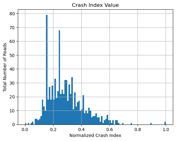

1.13 Plot an interactive map of the street networks, colored by the crash index

You can use GeoPandas to make an interactive Folium map, coloring the streets by the crash index column.

Tip: if you use the viridis color map, try using a “dark” tile set for better constrast of the colors.

import folium

m = merged_CPD.explore(
    column="crash_index_normalized",
    tiles="Cartodb dark matter",
)
m

Make this Notebook Trusted to load map: File -> Trust Notebook

Part 2: Scraping Craigslist

In this part, we’ll be extracting information on apartments from Craigslist search results. You’ll be using Selenium and BeautifulSoup to extract the relevant information from the HTML text.

For reference on CSS selectors, please see the notes from Week 6.

Primer: the Craigslist website URL

We’ll start with the Philadelphia region. First we need to figure out how to submit a query to Craigslist. As with many websites, one way you can do this is simply by constructing the proper URL and sending it to Craigslist.

https://philadelphia.craigslist.org/search/apa?min_price=1&min_bedrooms=1&minSqft=1#search=1_gallery0~0

There are three components to this URL.

The base URL: http://philadelphia.craigslist.org/search/apa
The user’s search parameters: ?min_price=1&min_bedrooms=1&minSqft=1

We will send nonzero defaults for some parameters (bedrooms, size, price) in order to exclude results that have empty values for these parameters.

The URL hash: #search=1~gallery~0~0

As we will see later, this part will be important because it contains the search page result number.

The Craigslist website requires Javascript, so we’ll need to use Selenium to load the page, and then use BeautifulSoup to extract the information we want.

2.1 Initialize a selenium driver and open Craigslist

As discussed in lecture, you can use Chrome, Firefox, or Edge as your selenium driver. In this part, you should do two things:

Initialize the selenium driver
Use the driver.get() function to open the following URL:

https://philadelphia.craigslist.org/search/apa?min_price=1&min_bedrooms=1&minSqft=1#search=1_gallery0~0

This will give you the search results for 1-bedroom apartments in Philadelphia.

from selenium import webdriver
from bs4 import BeautifulSoup
import requests
from selenium.webdriver.common.by import By
import pandas as pd

driver = webdriver.Chrome()

C:\Users\Owner\AppData\Local\Temp\ipykernel_25652\537431734.py:1: ResourceWarning: unclosed file <_io.BufferedWriter name='nul'>
  driver = webdriver.Chrome()

url = "https://philadelphia.craigslist.org/search/apa?min_price=1&min_bedrooms=1&minSqft=1#search=1gallery0~0"
driver.get(url)

2.2 Initialize your “soup”

Once selenium has the page open, we can get the page source from the driver and use BeautifulSoup to parse it. In this part, initialize a BeautifulSoup object with the driver’s page source

propertySoup = BeautifulSoup(driver.page_source, "html.parser")

2.3 Parsing the HTML

Now that we have our “soup” object, we can use BeautifulSoup to extract out the elements we need:

Use the Web Inspector to identify the HTML element that holds the information on each apartment listing.
Use BeautifulSoup to extract these elements from the HTML.

At the end of this part, you should have a list of 120 elements, where each element is the listing for a specific apartment on the search page.

element = propertySoup.select("li.cl-search-result")

#element

len(element)

print(element[0].prettify())
print(len(element))

<li class="cl-search-result cl-search-view-mode-gallery" data-pid="7678961565" title="A fresh take on living: Explore our 1 BR, 680 Sq Ft spaces.">
 <div class="gallery-card">
  <div class="cl-gallery">
   <div class="gallery-inner">
    <a class="main" href="https://philadelphia.craigslist.org/apa/d/north-wales-fresh-take-on-living/7678961565.html">
     <div class="swipe" style="visibility: visible;">
      <div class="swipe-wrap" style="width: 6768px;">
       <div data-index="0" style="width: 376px; left: 0px; transition-duration: 0ms; transform: translateX(0px);">
        <span class="loading icom-">
        </span>
        <img alt="A fresh take on living: Explore our 1 BR, 680 Sq Ft spaces. 1" src="https://images.craigslist.org/00Z0Z_g553W757i6Y_0ew09G_300x300.jpg"/>
       </div>
       <div data-index="1" style="width: 376px; left: -376px; transition-duration: 0ms; transform: translateX(376px);">
       </div>
       <div data-index="2" style="width: 376px; left: -752px; transition-duration: 0ms; transform: translateX(376px);">
       </div>
       <div data-index="3" style="width: 376px; left: -1128px; transition-duration: 0ms; transform: translateX(376px);">
       </div>
       <div data-index="4" style="width: 376px; left: -1504px; transition-duration: 0ms; transform: translateX(376px);">
       </div>
       <div data-index="5" style="width: 376px; left: -1880px; transition-duration: 0ms; transform: translateX(376px);">
       </div>
       <div data-index="6" style="width: 376px; left: -2256px; transition-duration: 0ms; transform: translateX(376px);">
       </div>
       <div data-index="7" style="width: 376px; left: -2632px; transition-duration: 0ms; transform: translateX(376px);">
       </div>
       <div data-index="8" style="width: 376px; left: -3008px; transition-duration: 0ms; transform: translateX(-376px);">
       </div>
      </div>
     </div>
     <div class="slider-back-arrow icom-">
     </div>
     <div class="slider-forward-arrow icom-">
     </div>
    </a>
   </div>
   <div class="dots">
    <span class="dot selected">
     •
    </span>
    <span class="dot">
     •
    </span>
    <span class="dot">
     •
    </span>
    <span class="dot">
     •
    </span>
    <span class="dot">
     •
    </span>
    <span class="dot">
     •
    </span>
    <span class="dot">
     •
    </span>
    <span class="dot">
     •
    </span>
    <span class="dot">
     •
    </span>
   </div>
  </div>
  <a class="cl-app-anchor text-only posting-title" href="https://philadelphia.craigslist.org/apa/d/north-wales-fresh-take-on-living/7678961565.html" tabindex="0">
   <span class="label">
    A fresh take on living: Explore our 1 BR, 680 Sq Ft spaces.
   </span>
  </a>
  <div class="meta">
   14 mins ago
   <span class="separator">
    ·
   </span>
   <span class="housing-meta">
    <span class="post-bedrooms">
     1br
    </span>
    <span class="post-sqft">
     680ft
     <span class="exponent">
      2
     </span>
    </span>
   </span>
   <span class="separator">
    ·
   </span>
   North Wales, Lansdale, Horsham, Doylestown, Ambler
  </div>
  <span class="priceinfo">
   $1,722
  </span>
  <button class="bd-button cl-favorite-button icon-only" tabindex="0" title="add to favorites list" type="button">
   <span class="icon icom-">
   </span>
   <span class="label">
   </span>
  </button>
  <button class="bd-button cl-banish-button icon-only" tabindex="0" title="hide posting" type="button">
   <span class="icon icom-">
   </span>
   <span class="label">
    hide
   </span>
  </button>
 </div>
</li>

120

2.4 Find the relevant pieces of information

We will now focus on the first element in the list of 120 apartments. Use the prettify() function to print out the HTML for this first element.

From this HTML, identify the HTML elements that hold:

The apartment price
The number of bedrooms
The square footage
The apartment title

For the first apartment, print out each of these pieces of information, using BeautifulSoup to select the proper elements.

apt1 = element[0]
spans = apt1.select('span')
print(f"apartment price: {apt1.find('span',{'class' : 'priceinfo'}).text}",end="\n")

print(f"number of bedrooms: {apt1.find('span',{'class' : 'post-bedrooms'}).text[:1]}",end="\n")

print(f"square footage: {apt1.find('span',{'class' : 'post-sqft'}).text[:3]}",end="\n")

print(f"apartment title: {apt1.find('span',{'class' : 'label'}).text}",end="\n")

apartment price: $1,722
number of bedrooms: 1
square footage: 680
apartment title: A fresh take on living: Explore our 1 BR, 680 Sq Ft spaces.

2.5 Functions to format the results

In this section, you’ll create functions that take in the raw string elements for price, size, and number of bedrooms and returns them formatted as numbers.

I’ve started the functions to format the values. You should finish theses functions in this section.

Hints - You can use string formatting functions like string.replace() and string.strip() - The int() and float() functions can convert strings to numbers

def format_bedrooms(bedrooms_string):
    # Format the bedrooms string and return an int
    # 
    # This will involve using the string.replace() function to 
    # remove unwanted characters
    
    return int(bedrooms_string.replace("br",""))

def format_size(size_string):
    # Format the size string and return a float
    # 
    # This will involve using the string.replace() function to 
    # remove unwanted characters
    
    return float(f"{size_string[:-3]}")

def format_price(price_string):
    # Format the price string and return a float
    # 
    # This will involve using the string.strip() function to 
    # remove unwanted characters
    return float(price_string.replace("$","").replace(",",""))

2.6 Putting it all together

In this part, you’ll complete the code block below using results from previous parts. The code will loop over 5 pages of search results and scrape data for 600 apartments.

We can get a specific page by changing the search=PAGE part of the URL hash. For example, to get page 2 instead of page 1, we will navigate to:

https://philadelphia.craigslist.org/search/apa?min_price=1&min_bedrooms=1&minSqft=1#search=2_gallery0~0

In the code below, the outer for loop will loop over 5 pages of search results. The inner for loop will loop over the 120 apartments listed on each search page.

Fill in the missing pieces of the inner loop using the code from the previous section. We will be able to extract out the relevant pieces of info for each apartment.

After filling in the missing pieces and executing the code cell, you should have a Data Frame called results that holds the data for 600 apartment listings.

Notes

Be careful if you try to scrape more listings. Craigslist will temporarily ban your IP address (for a very short time) if you scrape too much at once. I’ve added a sleep() function to the for loop to wait 30 seconds between scraping requests.

If the for loop gets stuck at the “Processing page X…” step for more than a minute or so, your IP address is probably banned temporarily, and you’ll have to wait a few minutes before trying again.

from time import sleep

results = []

# search in batches of 120 for 5 pages
# NOTE: you will get temporarily banned if running more than ~5 pages or so
# the API limits are more leninient during off-peak times, and you can try
# experimenting with more pages
max_pages = 5

# The base URL we will be using
base_url = "https://philadelphia.craigslist.org/search/apa?min_price=1&min_bedrooms=1&minSqft=1"

# loop over each page of search results
for page_num in range(1, max_pages + 1):
    print(f"Processing page {page_num}...")

    # Update the URL hash for this page number and make the combined URL
    url_hash = f"#search={page_num}~gallery~0~0"
    url = base_url + url_hash

    # Go to the driver and wait for 5 seconds
    driver.get(url)
    sleep(5)

    # YOUR CODE: get the list of all apartments
    # This is the same code from Part 1.2 and 1.3
    # It should be a list of 120 apartments
    soup = BeautifulSoup(driver.page_source,"html.parser")
    apts = soup.select("li.cl-search-result")
    print("Number of apartments = ", len(apts))

    # loop over each apartment in the list
    page_results = []
    for apt in apts:

        # YOUR CODE: the bedrooms string
        bedrooms = format_bedrooms(apt.find('span',{'class' : 'post-bedrooms'}).text)

        # YOUR CODE: the size string
        size = format_size(apt.find('span',{'class' : 'post-sqft'}).text)

        # YOUR CODE: the title string
        title = apt.find('span',{'class' : 'label'}).text

        # YOUR CODE: the price string
        price = format_price(apt.find('span',{'class' : 'priceinfo'}).text)


        # Format using functions from Part 1.5
        # bedrooms = format_bedrooms(bedrooms)
        # size = format_size(size)
        # price = format_price(price)

        # Save the result
        page_results.append([price, size, bedrooms, title])

    # Create a dataframe and save
    col_names = ["price", "size", "bedrooms", "title"]
    df = pd.DataFrame(page_results, columns=col_names)
    results.append(df)

    print("sleeping for 10 seconds between calls")
    sleep(10)

# Finally, concatenate all the results
results = pd.concat(results, axis=0).reset_index(drop=True)

Processing page 1...
Number of apartments =  120
sleeping for 10 seconds between calls
Processing page 2...
Number of apartments =  120
sleeping for 10 seconds between calls
Processing page 3...
Number of apartments =  120
sleeping for 10 seconds between calls
Processing page 4...
Number of apartments =  120
sleeping for 10 seconds between calls
Processing page 5...
Number of apartments =  120
sleeping for 10 seconds between calls

results.head(4)

	price	size	bedrooms	title
0	1722.0	680.0	1	A fresh take on living: Explore our 1 BR, 680 ...
1	850.0	400.0	1	Cozy and clean apartment
2	1905.0	926.0	2	2 bedroom, 9' Ceilings w/ Crown Molding, West ...
3	1788.0	521.0	1	1/bd, Conference Room, Fully Equipped Kitchens

2.7 Plotting the distribution of prices

Use matplotlib’s hist() function to make two histograms for:

Apartment prices
Apartment prices per square foot (price / size)

Make sure to add labels to the respective axes and a title describing the plot.

fig,ax = plt.subplots(1,1)
ax.hist(
    results["price"],
    rwidth=0.65,
)
ax.set_title("Philadelphia Rental Apartment Price Frequencies - Source: Craigslist")
ax.set_xlabel("Listing Price ($)")
ax.set_ylabel("Frequency")

plt.show()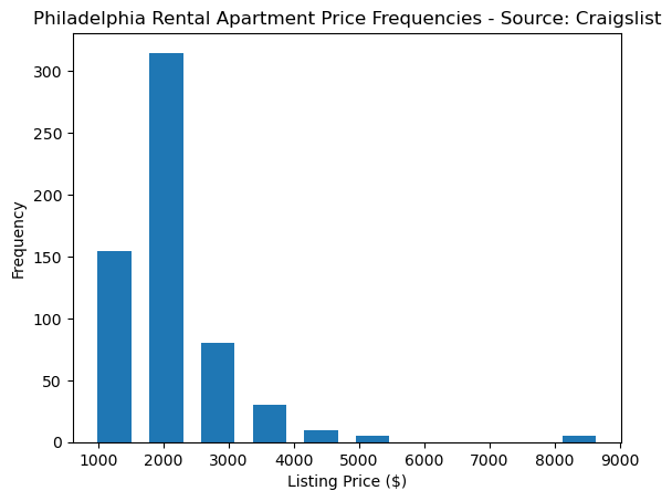

Side note: rental prices per sq. ft. from Craigslist

The histogram of price per sq ft should be centered around ~1.5. Here is a plot of how Philadelphia’s rents compare to the other most populous cities:

Source

fig,ax = plt.subplots(1,1)
ax.hist(
    results["price"]/results["size"],
    rwidth=0.65
)

ax.set_title("Price per Sq. Ft. of Philadelphia Rental Apartments - Source: Craigslist")
ax.set_xlabel("Listing Price ($/sq. ft.)")
ax.set_ylabel("Frequency")

plt.show()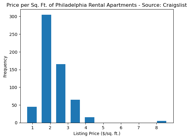

2.8 Comparing prices for different sizes

Use altair to explore the relationship between price, size, and number of bedrooms. Make an interactive scatter plot of price (x-axis) vs. size (y-axis), with the points colored by the number of bedrooms.

Make sure the plot is interactive (zoom-able and pan-able) and add a tooltip with all of the columns in our scraped data frame.

With this sort of plot, you can quickly see the outlier apartments in terms of size and price.

import altair as alt

colormap = alt.Scale(
    domain=[0,1,2,3,4,5],
    range=[
        "steelblue",
        "cornflowerblue",
        "chartreuse",
        "#F4D03F",
        "#D35400",
        "red",
    ])

# Step 1: Initialize the chart with the data
scatter = alt.Chart(results).mark_circle(size=50).encode(
    x=alt.X('price:Q'),
    y=alt.Y('size:Q'),
    color=alt.Color('bedrooms:Q',sort="ascending",scale=colormap),
    tooltip=["title", "price","size","bedrooms"],
).properties(width=350,height=150)

scatter.interactive()