import pandas as pd
import geopandas as gpd
import numpy as np
import hvplot.pandas
import matplotlib.pyplot as plt
import rasterio as rio
pd.options.display.max_columns = 999
# Hide warnings due to issue in shapely package
# See: https://github.com/shapely/shapely/issues/1345
np.seterr(invalid="ignore");Exploring Evictions and Code Violations in Philadelphia
This assignment will contain two parts:
- Exploring evictions and code violations in Philadelphia
- Comparing the NDVI in Philadelphia
Part 1: Exploring Evictions and Code Violations in Philadelphia
In this assignment, we’ll explore spatial trends evictions in Philadelphia using data from the Eviction Lab and building code violations using data from OpenDataPhilly.
We’ll be exploring the idea that evictions can occur as retaliation against renters for reporting code violations. Spatial correlations between evictions and code violations from the City’s Licenses and Inspections department can offer some insight into this question.
A couple of interesting background readings: - HuffPost article - PlanPhilly article
1.1 Explore Eviction Lab Data
The Eviction Lab built the first national database for evictions. If you aren’t familiar with the project, you can explore their website: https://evictionlab.org/
1.1.1 Read data using geopandas
The first step is to read the eviction data by census tract using geopandas. The data for all of Pennsylvania by census tract is available in the data/ folder in a GeoJSON format.
Load the data file “PA-tracts.geojson” using geopandas
Note: If you’d like to see all columns in the data frame, you can increase the max number of columns using pandas display options:
CityLimitsdf = gpd.read_file("./Data/City_Limits.geojson")
PATractsdf = gpd.read_file("./Data/PA-tracts.geojson")
pprTreePoints = gpd.read_file("./Data/ppr_tree_canopy_points_2015.geojson")#CityLimitsdf.head()
#PATractsdf.head()
#pprTreePoints.head(5)1.1.2 Explore and trim the data
We will need to trim data to Philadelphia only. Take a look at the data dictionary for the descriptions of the various columns in top-level repository folder: eviction_lab_data_dictionary.txt
Note: the column names are shortened — see the end of the above file for the abbreviations. The numbers at the end of the columns indicate the years. For example, e-16 is the number of evictions in 2016.
Take a look at the individual columns and trim to census tracts in Philadelphia. (Hint: Philadelphia is both a city and a county).
tracts_filtered = PATractsdf[PATractsdf['pl'].str.startswith('Philadelphia')]tracts_filtered.head()| GEOID | west | south | east | north | n | pl | p-00 | pr-00 | roh-00 | pro-00 | mgr-00 | mhi-00 | mpv-00 | rb-00 | pw-00 | paa-00 | ph-00 | pai-00 | pa-00 | pnp-00 | pm-00 | po-00 | ef-00 | e-00 | er-00 | efr-00 | lf-00 | imputed-00 | subbed-00 | p-01 | pr-01 | roh-01 | pro-01 | mgr-01 | mhi-01 | mpv-01 | rb-01 | pw-01 | paa-01 | ph-01 | pai-01 | pa-01 | pnp-01 | pm-01 | po-01 | ef-01 | e-01 | er-01 | efr-01 | lf-01 | imputed-01 | subbed-01 | p-02 | pr-02 | roh-02 | pro-02 | mgr-02 | mhi-02 | mpv-02 | rb-02 | pw-02 | paa-02 | ph-02 | pai-02 | pa-02 | pnp-02 | pm-02 | po-02 | ef-02 | e-02 | er-02 | efr-02 | lf-02 | imputed-02 | subbed-02 | p-03 | pr-03 | roh-03 | pro-03 | mgr-03 | mhi-03 | mpv-03 | rb-03 | pw-03 | paa-03 | ph-03 | pai-03 | pa-03 | pnp-03 | pm-03 | po-03 | ef-03 | e-03 | er-03 | efr-03 | lf-03 | imputed-03 | subbed-03 | p-04 | pr-04 | roh-04 | pro-04 | mgr-04 | mhi-04 | mpv-04 | rb-04 | pw-04 | paa-04 | ph-04 | pai-04 | pa-04 | pnp-04 | pm-04 | po-04 | ef-04 | e-04 | er-04 | efr-04 | lf-04 | imputed-04 | subbed-04 | p-05 | pr-05 | roh-05 | pro-05 | mgr-05 | mhi-05 | mpv-05 | rb-05 | pw-05 | paa-05 | ph-05 | pai-05 | pa-05 | pnp-05 | pm-05 | po-05 | ef-05 | e-05 | er-05 | efr-05 | lf-05 | imputed-05 | subbed-05 | p-06 | pr-06 | roh-06 | pro-06 | mgr-06 | mhi-06 | mpv-06 | rb-06 | pw-06 | paa-06 | ph-06 | pai-06 | pa-06 | pnp-06 | pm-06 | po-06 | ef-06 | e-06 | er-06 | efr-06 | lf-06 | imputed-06 | subbed-06 | p-07 | pr-07 | roh-07 | pro-07 | mgr-07 | mhi-07 | mpv-07 | rb-07 | pw-07 | paa-07 | ph-07 | pai-07 | pa-07 | pnp-07 | pm-07 | po-07 | ef-07 | e-07 | er-07 | efr-07 | lf-07 | imputed-07 | subbed-07 | p-08 | pr-08 | roh-08 | pro-08 | mgr-08 | mhi-08 | mpv-08 | rb-08 | pw-08 | paa-08 | ph-08 | pai-08 | pa-08 | pnp-08 | pm-08 | po-08 | ef-08 | e-08 | er-08 | efr-08 | lf-08 | imputed-08 | subbed-08 | p-09 | pr-09 | roh-09 | pro-09 | mgr-09 | mhi-09 | mpv-09 | rb-09 | pw-09 | paa-09 | ph-09 | pai-09 | pa-09 | pnp-09 | pm-09 | po-09 | ef-09 | e-09 | er-09 | efr-09 | lf-09 | imputed-09 | subbed-09 | p-10 | pr-10 | roh-10 | pro-10 | mgr-10 | mhi-10 | mpv-10 | rb-10 | pw-10 | paa-10 | ph-10 | pai-10 | pa-10 | pnp-10 | pm-10 | po-10 | ef-10 | e-10 | er-10 | efr-10 | lf-10 | imputed-10 | subbed-10 | p-11 | pr-11 | roh-11 | pro-11 | mgr-11 | mhi-11 | mpv-11 | rb-11 | pw-11 | paa-11 | ph-11 | pai-11 | pa-11 | pnp-11 | pm-11 | po-11 | ef-11 | e-11 | er-11 | efr-11 | lf-11 | imputed-11 | subbed-11 | p-12 | pr-12 | roh-12 | pro-12 | mgr-12 | mhi-12 | mpv-12 | rb-12 | pw-12 | paa-12 | ph-12 | pai-12 | pa-12 | pnp-12 | pm-12 | po-12 | ef-12 | e-12 | er-12 | efr-12 | lf-12 | imputed-12 | subbed-12 | p-13 | pr-13 | roh-13 | pro-13 | mgr-13 | mhi-13 | mpv-13 | rb-13 | pw-13 | paa-13 | ph-13 | pai-13 | pa-13 | pnp-13 | pm-13 | po-13 | ef-13 | e-13 | er-13 | efr-13 | lf-13 | imputed-13 | subbed-13 | p-14 | pr-14 | roh-14 | pro-14 | mgr-14 | mhi-14 | mpv-14 | rb-14 | pw-14 | paa-14 | ph-14 | pai-14 | pa-14 | pnp-14 | pm-14 | po-14 | ef-14 | e-14 | er-14 | efr-14 | lf-14 | imputed-14 | subbed-14 | p-15 | pr-15 | roh-15 | pro-15 | mgr-15 | mhi-15 | mpv-15 | rb-15 | pw-15 | paa-15 | ph-15 | pai-15 | pa-15 | pnp-15 | pm-15 | po-15 | ef-15 | e-15 | er-15 | efr-15 | lf-15 | imputed-15 | subbed-15 | p-16 | pr-16 | roh-16 | pro-16 | mgr-16 | mhi-16 | mpv-16 | rb-16 | pw-16 | paa-16 | ph-16 | pai-16 | pa-16 | pnp-16 | pm-16 | po-16 | ef-16 | e-16 | er-16 | efr-16 | lf-16 | imputed-16 | subbed-16 | geometry | |
|---|---|---|---|---|---|---|---|---|---|---|---|---|---|---|---|---|---|---|---|---|---|---|---|---|---|---|---|---|---|---|---|---|---|---|---|---|---|---|---|---|---|---|---|---|---|---|---|---|---|---|---|---|---|---|---|---|---|---|---|---|---|---|---|---|---|---|---|---|---|---|---|---|---|---|---|---|---|---|---|---|---|---|---|---|---|---|---|---|---|---|---|---|---|---|---|---|---|---|---|---|---|---|---|---|---|---|---|---|---|---|---|---|---|---|---|---|---|---|---|---|---|---|---|---|---|---|---|---|---|---|---|---|---|---|---|---|---|---|---|---|---|---|---|---|---|---|---|---|---|---|---|---|---|---|---|---|---|---|---|---|---|---|---|---|---|---|---|---|---|---|---|---|---|---|---|---|---|---|---|---|---|---|---|---|---|---|---|---|---|---|---|---|---|---|---|---|---|---|---|---|---|---|---|---|---|---|---|---|---|---|---|---|---|---|---|---|---|---|---|---|---|---|---|---|---|---|---|---|---|---|---|---|---|---|---|---|---|---|---|---|---|---|---|---|---|---|---|---|---|---|---|---|---|---|---|---|---|---|---|---|---|---|---|---|---|---|---|---|---|---|---|---|---|---|---|---|---|---|---|---|---|---|---|---|---|---|---|---|---|---|---|---|---|---|---|---|---|---|---|---|---|---|---|---|---|---|---|---|---|---|---|---|---|---|---|---|---|---|---|---|---|---|---|---|---|---|---|---|---|---|---|---|---|---|---|---|---|---|---|---|---|---|---|---|---|---|---|---|---|---|---|---|---|---|---|---|---|---|---|---|---|---|---|---|---|---|---|---|---|---|---|---|---|---|---|---|---|---|---|---|---|---|---|---|---|---|---|---|---|---|---|---|---|---|---|---|---|---|---|
| 435 | 42101000100 | -75.1523 | 39.9481 | -75.1415 | 39.9569 | 1 | Philadelphia County, Pennsylvania | 2646.71 | 9.26 | 1347.0 | 77.12 | 959.0 | 48886.0 | 189700.0 | 24.5 | 78.45 | 12.42 | 3.47 | 0.23 | 3.92 | 0.00 | 1.40 | 0.11 | NaN | NaN | NaN | NaN | 0.0 | 0.0 | 0.0 | 2646.71 | 9.26 | 1360.0 | 77.12 | 959.0 | 48886.0 | 189700.0 | 24.5 | 78.45 | 12.42 | 3.47 | 0.23 | 3.92 | 0.00 | 1.40 | 0.11 | NaN | NaN | NaN | NaN | 0.0 | 0.0 | 0.0 | 2646.71 | 9.26 | 1374.0 | 77.12 | 959.0 | 48886.0 | 189700.0 | 24.5 | 78.45 | 12.42 | 3.47 | 0.23 | 3.92 | 0.00 | 1.40 | 0.11 | 21.0 | 19.0 | 1.38 | 1.53 | 1.0 | 0.0 | 0.0 | 2646.71 | 9.26 | 1388.0 | 77.12 | 959.0 | 48886.0 | 189700.0 | 24.5 | 78.45 | 12.42 | 3.47 | 0.23 | 3.92 | 0.00 | 1.40 | 0.11 | 25.0 | 21.0 | 1.51 | 1.80 | 1.0 | 0.0 | 0.0 | 2646.71 | 9.26 | 1401.0 | 77.12 | 959.0 | 48886.0 | 189700.0 | 24.5 | 78.45 | 12.42 | 3.47 | 0.23 | 3.92 | 0.00 | 1.40 | 0.11 | 25.0 | 24.0 | 1.71 | 1.78 | 1.0 | 0.0 | 0.0 | 3310.88 | 12.11 | 1415.0 | 57.97 | 1357.0 | 73272.0 | 332500.0 | 25.6 | 83.98 | 7.24 | 4.40 | 0.0 | 3.08 | 0.0 | 0.45 | 0.84 | 18.0 | 15.0 | 1.06 | 1.27 | 1.0 | 0.0 | 0.0 | 3310.88 | 12.11 | 1428.0 | 57.97 | 1357.0 | 73272.0 | 332500.0 | 25.6 | 83.98 | 7.24 | 4.40 | 0.0 | 3.08 | 0.0 | 0.45 | 0.84 | 13.0 | 10.0 | 0.70 | 0.91 | 1.0 | 0.0 | 0.0 | 3310.88 | 12.11 | 1442.0 | 57.97 | 1357.0 | 73272.0 | 332500.0 | 25.6 | 83.98 | 7.24 | 4.40 | 0.0 | 3.08 | 0.0 | 0.45 | 0.84 | 53.0 | 20.0 | 1.39 | 3.68 | 0.0 | 0.0 | 1.0 | 3310.88 | 12.11 | 1456.0 | 57.97 | 1357.0 | 73272.0 | 332500.0 | 25.6 | 83.98 | 7.24 | 4.40 | 0.0 | 3.08 | 0.0 | 0.45 | 0.84 | 30.0 | 17.0 | 1.17 | 2.06 | 0.0 | 0.0 | 1.0 | 3310.88 | 12.11 | 1469.0 | 57.97 | 1357.0 | 73272.0 | 332500.0 | 25.6 | 83.98 | 7.24 | 4.40 | 0.0 | 3.08 | 0.0 | 0.45 | 0.84 | 25.0 | 11.0 | 0.75 | 1.70 | 0.0 | 0.0 | 1.0 | 3478.0 | 3.13 | 1483.0 | 64.45 | 1491.0 | 75505.0 | 340800.0 | 27.5 | 83.09 | 5.95 | 3.62 | 0.14 | 4.97 | 0.06 | 2.01 | 0.14 | 24.0 | 18.0 | 1.21 | 1.62 | 0.0 | 0.0 | 1.0 | 3608.0 | 0.00 | 1524.0 | 71.19 | 1545.0 | 92207.0 | 351600.0 | 24.3 | 73.45 | 10.01 | 5.10 | 0.17 | 8.79 | 0.0 | 2.49 | 0.00 | 23.0 | 11.0 | 0.72 | 1.51 | 0.0 | 0.0 | 1.0 | 3608.0 | 0.00 | 1565.0 | 71.19 | 1545.0 | 92207.0 | 351600.0 | 24.3 | 73.45 | 10.01 | 5.10 | 0.17 | 8.79 | 0.0 | 2.49 | 0.00 | 22.0 | 7.0 | 0.45 | 1.41 | 0.0 | 0.0 | 1.0 | 3608.0 | 0.00 | 1606.0 | 71.19 | 1545.0 | 92207.0 | 351600.0 | 24.3 | 73.45 | 10.01 | 5.10 | 0.17 | 8.79 | 0.0 | 2.49 | 0.00 | 25.0 | 12.0 | 0.75 | 1.56 | 0.0 | 0.0 | 1.0 | 3608.0 | 0.00 | 1646.0 | 71.19 | 1545.0 | 92207.0 | 351600.0 | 24.3 | 73.45 | 10.01 | 5.10 | 0.17 | 8.79 | 0.0 | 2.49 | 0.00 | 26.0 | 12.0 | 0.73 | 1.58 | 0.0 | 0.0 | 1.0 | 3608.0 | 0.00 | 1687.0 | 71.19 | 1545.0 | 92207.0 | 351600.0 | 24.3 | 73.45 | 10.01 | 5.10 | 0.17 | 8.79 | 0.0 | 2.49 | 0.00 | 31.0 | 12.0 | 0.71 | 1.84 | 0.0 | 0.0 | 1.0 | 3608.0 | 0.00 | 1728.0 | 71.19 | 1545.0 | 92207.0 | 351600.0 | 24.3 | 73.45 | 10.01 | 5.10 | 0.17 | 8.79 | 0.0 | 2.49 | 0.00 | 25.0 | 16.0 | 0.93 | 1.45 | 0.0 | 0.0 | 1.0 | MULTIPOLYGON (((-75.14161 39.95549, -75.14163 ... |
| 436 | 42101000200 | -75.1631 | 39.9529 | -75.1511 | 39.9578 | 2 | Philadelphia County, Pennsylvania | 1362.00 | 56.42 | 374.0 | 81.48 | 421.0 | 8349.0 | 55600.0 | 31.2 | 11.16 | 5.21 | 1.69 | 0.07 | 79.59 | 0.07 | 2.20 | 0.00 | NaN | NaN | NaN | NaN | 0.0 | 0.0 | 0.0 | 1362.00 | 56.42 | 415.0 | 81.48 | 421.0 | 8349.0 | 55600.0 | 31.2 | 11.16 | 5.21 | 1.69 | 0.07 | 79.59 | 0.07 | 2.20 | 0.00 | NaN | NaN | NaN | NaN | 0.0 | 0.0 | 0.0 | 1362.00 | 56.42 | 455.0 | 81.48 | 421.0 | 8349.0 | 55600.0 | 31.2 | 11.16 | 5.21 | 1.69 | 0.07 | 79.59 | 0.07 | 2.20 | 0.00 | 4.0 | 4.0 | 0.88 | 0.88 | 1.0 | 0.0 | 0.0 | 1362.00 | 56.42 | 496.0 | 81.48 | 421.0 | 8349.0 | 55600.0 | 31.2 | 11.16 | 5.21 | 1.69 | 0.07 | 79.59 | 0.07 | 2.20 | 0.00 | 3.0 | 3.0 | 0.60 | 0.60 | 1.0 | 0.0 | 0.0 | 1362.00 | 56.42 | 537.0 | 81.48 | 421.0 | 8349.0 | 55600.0 | 31.2 | 11.16 | 5.21 | 1.69 | 0.07 | 79.59 | 0.07 | 2.20 | 0.00 | 6.0 | 6.0 | 1.12 | 1.12 | 1.0 | 0.0 | 0.0 | 1633.00 | 3.45 | 578.0 | 56.04 | 675.0 | 42083.0 | 232800.0 | 24.7 | 19.29 | 2.82 | 1.22 | 0.0 | 76.00 | 0.0 | 0.67 | 0.00 | 1.0 | 0.0 | 0.00 | 0.17 | 1.0 | 0.0 | 0.0 | 1633.00 | 3.45 | 618.0 | 56.04 | 675.0 | 42083.0 | 232800.0 | 24.7 | 19.29 | 2.82 | 1.22 | 0.0 | 76.00 | 0.0 | 0.67 | 0.00 | 6.0 | 6.0 | 0.97 | 0.97 | 1.0 | 0.0 | 0.0 | 1633.00 | 3.45 | 659.0 | 56.04 | 675.0 | 42083.0 | 232800.0 | 24.7 | 19.29 | 2.82 | 1.22 | 0.0 | 76.00 | 0.0 | 0.67 | 0.00 | 9.0 | 7.0 | 1.06 | 1.37 | 0.0 | 0.0 | 1.0 | 1633.00 | 3.45 | 700.0 | 56.04 | 675.0 | 42083.0 | 232800.0 | 24.7 | 19.29 | 2.82 | 1.22 | 0.0 | 76.00 | 0.0 | 0.67 | 0.00 | 11.0 | 7.0 | 1.00 | 1.57 | 0.0 | 0.0 | 1.0 | 1633.00 | 3.45 | 740.0 | 56.04 | 675.0 | 42083.0 | 232800.0 | 24.7 | 19.29 | 2.82 | 1.22 | 0.0 | 76.00 | 0.0 | 0.67 | 0.00 | 6.0 | 5.0 | 0.68 | 0.81 | 0.0 | 0.0 | 1.0 | 2937.0 | 5.07 | 781.0 | 68.21 | 905.0 | 49928.0 | 261100.0 | 26.4 | 22.64 | 9.67 | 2.69 | 0.10 | 63.16 | 0.03 | 1.40 | 0.31 | 6.0 | 1.0 | 0.13 | 0.77 | 0.0 | 0.0 | 1.0 | 2331.0 | 15.78 | 792.0 | 60.27 | 1263.0 | 59891.0 | 265400.0 | 28.1 | 38.91 | 6.05 | 1.54 | 0.47 | 50.75 | 0.0 | 2.27 | 0.00 | 9.0 | 6.0 | 0.76 | 1.14 | 0.0 | 0.0 | 1.0 | 2331.0 | 15.78 | 802.0 | 60.27 | 1263.0 | 59891.0 | 265400.0 | 28.1 | 38.91 | 6.05 | 1.54 | 0.47 | 50.75 | 0.0 | 2.27 | 0.00 | 8.0 | 3.0 | 0.37 | 1.00 | 0.0 | 0.0 | 1.0 | 2331.0 | 15.78 | 813.0 | 60.27 | 1263.0 | 59891.0 | 265400.0 | 28.1 | 38.91 | 6.05 | 1.54 | 0.47 | 50.75 | 0.0 | 2.27 | 0.00 | 14.0 | 10.0 | 1.23 | 1.72 | 0.0 | 0.0 | 1.0 | 2331.0 | 15.78 | 824.0 | 60.27 | 1263.0 | 59891.0 | 265400.0 | 28.1 | 38.91 | 6.05 | 1.54 | 0.47 | 50.75 | 0.0 | 2.27 | 0.00 | 5.0 | 3.0 | 0.36 | 0.61 | 0.0 | 0.0 | 1.0 | 2331.0 | 15.78 | 834.0 | 60.27 | 1263.0 | 59891.0 | 265400.0 | 28.1 | 38.91 | 6.05 | 1.54 | 0.47 | 50.75 | 0.0 | 2.27 | 0.00 | 10.0 | 9.0 | 1.08 | 1.20 | 0.0 | 0.0 | 1.0 | 2331.0 | 15.78 | 845.0 | 60.27 | 1263.0 | 59891.0 | 265400.0 | 28.1 | 38.91 | 6.05 | 1.54 | 0.47 | 50.75 | 0.0 | 2.27 | 0.00 | 11.0 | 8.0 | 0.95 | 1.30 | 0.0 | 0.0 | 1.0 | MULTIPOLYGON (((-75.15122 39.95686, -75.15167 ... |
| 437 | 42101000300 | -75.1798 | 39.9544 | -75.1623 | 39.9599 | 3 | Philadelphia County, Pennsylvania | 2570.00 | 12.16 | 861.0 | 69.49 | 688.0 | 40625.0 | 233900.0 | 29.0 | 70.86 | 14.67 | 3.81 | 0.27 | 7.00 | 0.08 | 3.04 | 0.27 | NaN | NaN | NaN | NaN | 0.0 | 0.0 | 0.0 | 2570.00 | 12.16 | 915.0 | 69.49 | 688.0 | 40625.0 | 233900.0 | 29.0 | 70.86 | 14.67 | 3.81 | 0.27 | 7.00 | 0.08 | 3.04 | 0.27 | NaN | NaN | NaN | NaN | 0.0 | 0.0 | 0.0 | 2570.00 | 12.16 | 969.0 | 69.49 | 688.0 | 40625.0 | 233900.0 | 29.0 | 70.86 | 14.67 | 3.81 | 0.27 | 7.00 | 0.08 | 3.04 | 0.27 | 14.0 | 12.0 | 1.24 | 1.44 | 1.0 | 0.0 | 0.0 | 2570.00 | 12.16 | 1023.0 | 69.49 | 688.0 | 40625.0 | 233900.0 | 29.0 | 70.86 | 14.67 | 3.81 | 0.27 | 7.00 | 0.08 | 3.04 | 0.27 | 21.0 | 17.0 | 1.66 | 2.05 | 1.0 | 0.0 | 0.0 | 2570.00 | 12.16 | 1077.0 | 69.49 | 688.0 | 40625.0 | 233900.0 | 29.0 | 70.86 | 14.67 | 3.81 | 0.27 | 7.00 | 0.08 | 3.04 | 0.27 | 23.0 | 23.0 | 2.13 | 2.13 | 1.0 | 0.0 | 0.0 | 4497.00 | 1.63 | 1132.0 | 65.66 | 1184.0 | 59189.0 | 438500.0 | 24.8 | 67.44 | 10.52 | 5.69 | 0.2 | 14.14 | 0.0 | 1.29 | 0.71 | 12.0 | 10.0 | 0.88 | 1.06 | 1.0 | 0.0 | 0.0 | 4497.00 | 1.63 | 1186.0 | 65.66 | 1184.0 | 59189.0 | 438500.0 | 24.8 | 67.44 | 10.52 | 5.69 | 0.2 | 14.14 | 0.0 | 1.29 | 0.71 | 19.0 | 16.0 | 1.35 | 1.60 | 1.0 | 0.0 | 0.0 | 4497.00 | 1.63 | 1240.0 | 65.66 | 1184.0 | 59189.0 | 438500.0 | 24.8 | 67.44 | 10.52 | 5.69 | 0.2 | 14.14 | 0.0 | 1.29 | 0.71 | 21.0 | 7.0 | 0.56 | 1.69 | 0.0 | 0.0 | 1.0 | 4497.00 | 1.63 | 1294.0 | 65.66 | 1184.0 | 59189.0 | 438500.0 | 24.8 | 67.44 | 10.52 | 5.69 | 0.2 | 14.14 | 0.0 | 1.29 | 0.71 | 25.0 | 11.0 | 0.85 | 1.93 | 0.0 | 0.0 | 1.0 | 4497.00 | 1.63 | 1348.0 | 65.66 | 1184.0 | 59189.0 | 438500.0 | 24.8 | 67.44 | 10.52 | 5.69 | 0.2 | 14.14 | 0.0 | 1.29 | 0.71 | 27.0 | 12.0 | 0.89 | 2.00 | 0.0 | 0.0 | 1.0 | 3169.0 | 7.20 | 1402.0 | 75.58 | 1827.0 | 71250.0 | 451800.0 | 28.0 | 72.26 | 10.22 | 4.26 | 0.03 | 10.35 | 0.03 | 2.52 | 0.32 | 24.0 | 13.0 | 0.93 | 1.71 | 0.0 | 0.0 | 1.0 | 3405.0 | 4.17 | 1489.0 | 70.47 | 1938.0 | 81950.0 | 469900.0 | 26.2 | 72.19 | 5.26 | 8.75 | 0.00 | 12.04 | 0.0 | 1.76 | 0.00 | 21.0 | 8.0 | 0.54 | 1.41 | 0.0 | 0.0 | 1.0 | 3405.0 | 4.17 | 1575.0 | 70.47 | 1938.0 | 81950.0 | 469900.0 | 26.2 | 72.19 | 5.26 | 8.75 | 0.00 | 12.04 | 0.0 | 1.76 | 0.00 | 27.0 | 12.0 | 0.76 | 1.71 | 0.0 | 0.0 | 1.0 | 3405.0 | 4.17 | 1662.0 | 70.47 | 1938.0 | 81950.0 | 469900.0 | 26.2 | 72.19 | 5.26 | 8.75 | 0.00 | 12.04 | 0.0 | 1.76 | 0.00 | 31.0 | 10.0 | 0.60 | 1.87 | 0.0 | 0.0 | 1.0 | 3405.0 | 4.17 | 1749.0 | 70.47 | 1938.0 | 81950.0 | 469900.0 | 26.2 | 72.19 | 5.26 | 8.75 | 0.00 | 12.04 | 0.0 | 1.76 | 0.00 | 27.0 | 14.0 | 0.80 | 1.54 | 0.0 | 0.0 | 1.0 | 3405.0 | 4.17 | 1835.0 | 70.47 | 1938.0 | 81950.0 | 469900.0 | 26.2 | 72.19 | 5.26 | 8.75 | 0.00 | 12.04 | 0.0 | 1.76 | 0.00 | 18.0 | 5.0 | 0.27 | 0.98 | 0.0 | 0.0 | 1.0 | 3405.0 | 4.17 | 1922.0 | 70.47 | 1938.0 | 81950.0 | 469900.0 | 26.2 | 72.19 | 5.26 | 8.75 | 0.00 | 12.04 | 0.0 | 1.76 | 0.00 | 26.0 | 14.0 | 0.73 | 1.35 | 0.0 | 0.0 | 1.0 | MULTIPOLYGON (((-75.16234 39.95782, -75.16237 ... |
| 438 | 42101000801 | -75.1833 | 39.9486 | -75.1773 | 39.9515 | 8.01 | Philadelphia County, Pennsylvania | 1478.00 | 14.40 | 810.0 | 73.65 | 933.0 | 42346.0 | 265200.0 | 27.6 | 81.67 | 2.97 | 3.50 | 0.04 | 10.08 | 0.04 | 1.26 | 0.45 | NaN | NaN | NaN | NaN | 0.0 | 0.0 | 0.0 | 1478.00 | 14.40 | 801.0 | 73.65 | 933.0 | 42346.0 | 265200.0 | 27.6 | 81.67 | 2.97 | 3.50 | 0.04 | 10.08 | 0.04 | 1.26 | 0.45 | NaN | NaN | NaN | NaN | 0.0 | 0.0 | 0.0 | 1478.00 | 14.40 | 793.0 | 73.65 | 933.0 | 42346.0 | 265200.0 | 27.6 | 81.67 | 2.97 | 3.50 | 0.04 | 10.08 | 0.04 | 1.26 | 0.45 | 7.0 | 5.0 | 0.63 | 0.88 | 1.0 | 0.0 | 0.0 | 1478.00 | 14.40 | 784.0 | 73.65 | 933.0 | 42346.0 | 265200.0 | 27.6 | 81.67 | 2.97 | 3.50 | 0.04 | 10.08 | 0.04 | 1.26 | 0.45 | 19.0 | 13.0 | 1.66 | 2.42 | 1.0 | 0.0 | 0.0 | 1478.00 | 14.40 | 775.0 | 73.65 | 933.0 | 42346.0 | 265200.0 | 27.6 | 81.67 | 2.97 | 3.50 | 0.04 | 10.08 | 0.04 | 1.26 | 0.45 | 17.0 | 14.0 | 1.81 | 2.19 | 1.0 | 0.0 | 0.0 | 1344.37 | 11.10 | 767.0 | 66.11 | 1393.0 | 61590.0 | 431800.0 | 28.2 | 86.58 | 1.05 | 3.14 | 0.0 | 8.16 | 0.0 | 0.88 | 0.18 | 10.0 | 6.0 | 0.78 | 1.30 | 1.0 | 0.0 | 0.0 | 1344.37 | 11.10 | 758.0 | 66.11 | 1393.0 | 61590.0 | 431800.0 | 28.2 | 86.58 | 1.05 | 3.14 | 0.0 | 8.16 | 0.0 | 0.88 | 0.18 | 12.0 | 7.0 | 0.92 | 1.58 | 1.0 | 0.0 | 0.0 | 1344.37 | 11.10 | 749.0 | 66.11 | 1393.0 | 61590.0 | 431800.0 | 28.2 | 86.58 | 1.05 | 3.14 | 0.0 | 8.16 | 0.0 | 0.88 | 0.18 | 12.0 | 5.0 | 0.67 | 1.60 | 0.0 | 0.0 | 1.0 | 1344.37 | 11.10 | 740.0 | 66.11 | 1393.0 | 61590.0 | 431800.0 | 28.2 | 86.58 | 1.05 | 3.14 | 0.0 | 8.16 | 0.0 | 0.88 | 0.18 | 11.0 | 4.0 | 0.54 | 1.49 | 0.0 | 0.0 | 1.0 | 1344.37 | 11.10 | 732.0 | 66.11 | 1393.0 | 61590.0 | 431800.0 | 28.2 | 86.58 | 1.05 | 3.14 | 0.0 | 8.16 | 0.0 | 0.88 | 0.18 | 10.0 | 2.0 | 0.27 | 1.37 | 0.0 | 0.0 | 1.0 | 1562.0 | 2.46 | 723.0 | 71.09 | 2001.0 | 83125.0 | 459900.0 | 25.9 | 78.04 | 2.94 | 5.76 | 0.00 | 10.82 | 0.26 | 1.92 | 0.26 | 14.0 | 4.0 | 0.55 | 1.94 | 0.0 | 0.0 | 1.0 | 1692.0 | 3.25 | 734.0 | 74.87 | 2219.0 | 81620.0 | 656300.0 | 24.7 | 75.18 | 10.64 | 4.91 | 0.00 | 4.08 | 0.0 | 1.42 | 3.78 | 13.0 | 7.0 | 0.95 | 1.77 | 0.0 | 0.0 | 1.0 | 1692.0 | 3.25 | 746.0 | 74.87 | 2219.0 | 81620.0 | 656300.0 | 24.7 | 75.18 | 10.64 | 4.91 | 0.00 | 4.08 | 0.0 | 1.42 | 3.78 | 7.0 | 0.0 | 0.00 | 0.94 | 0.0 | 0.0 | 1.0 | 1692.0 | 3.25 | 757.0 | 74.87 | 2219.0 | 81620.0 | 656300.0 | 24.7 | 75.18 | 10.64 | 4.91 | 0.00 | 4.08 | 0.0 | 1.42 | 3.78 | 15.0 | 3.0 | 0.40 | 1.98 | 0.0 | 0.0 | 1.0 | 1692.0 | 3.25 | 768.0 | 74.87 | 2219.0 | 81620.0 | 656300.0 | 24.7 | 75.18 | 10.64 | 4.91 | 0.00 | 4.08 | 0.0 | 1.42 | 3.78 | 10.0 | 4.0 | 0.52 | 1.30 | 0.0 | 0.0 | 1.0 | 1692.0 | 3.25 | 780.0 | 74.87 | 2219.0 | 81620.0 | 656300.0 | 24.7 | 75.18 | 10.64 | 4.91 | 0.00 | 4.08 | 0.0 | 1.42 | 3.78 | 16.0 | 8.0 | 1.03 | 2.05 | 0.0 | 0.0 | 1.0 | 1692.0 | 3.25 | 791.0 | 74.87 | 2219.0 | 81620.0 | 656300.0 | 24.7 | 75.18 | 10.64 | 4.91 | 0.00 | 4.08 | 0.0 | 1.42 | 3.78 | 13.0 | 4.0 | 0.51 | 1.64 | 0.0 | 0.0 | 1.0 | MULTIPOLYGON (((-75.17732 39.95096, -75.17784 ... |
| 439 | 42101000804 | -75.1712 | 39.9470 | -75.1643 | 39.9501 | 8.04 | Philadelphia County, Pennsylvania | 3301.00 | 14.40 | 2058.0 | 73.65 | 933.0 | 42346.0 | 265200.0 | 27.6 | 81.67 | 2.97 | 3.50 | 0.04 | 10.08 | 0.04 | 1.26 | 0.45 | NaN | NaN | NaN | NaN | 0.0 | 0.0 | 0.0 | 3301.00 | 14.40 | 2050.0 | 73.65 | 933.0 | 42346.0 | 265200.0 | 27.6 | 81.67 | 2.97 | 3.50 | 0.04 | 10.08 | 0.04 | 1.26 | 0.45 | NaN | NaN | NaN | NaN | 0.0 | 0.0 | 0.0 | 3301.00 | 14.40 | 2042.0 | 73.65 | 933.0 | 42346.0 | 265200.0 | 27.6 | 81.67 | 2.97 | 3.50 | 0.04 | 10.08 | 0.04 | 1.26 | 0.45 | 22.0 | 18.0 | 0.88 | 1.08 | 1.0 | 0.0 | 0.0 | 3301.00 | 14.40 | 2033.0 | 73.65 | 933.0 | 42346.0 | 265200.0 | 27.6 | 81.67 | 2.97 | 3.50 | 0.04 | 10.08 | 0.04 | 1.26 | 0.45 | 31.0 | 21.0 | 1.03 | 1.52 | 1.0 | 0.0 | 0.0 | 3301.00 | 14.40 | 2025.0 | 73.65 | 933.0 | 42346.0 | 265200.0 | 27.6 | 81.67 | 2.97 | 3.50 | 0.04 | 10.08 | 0.04 | 1.26 | 0.45 | 18.0 | 15.0 | 0.74 | 0.89 | 1.0 | 0.0 | 0.0 | 3002.54 | 11.10 | 2017.0 | 66.11 | 1393.0 | 61590.0 | 431800.0 | 28.2 | 86.58 | 1.05 | 3.14 | 0.0 | 8.16 | 0.0 | 0.88 | 0.18 | 28.0 | 19.0 | 0.94 | 1.39 | 1.0 | 0.0 | 0.0 | 3002.54 | 11.10 | 2009.0 | 66.11 | 1393.0 | 61590.0 | 431800.0 | 28.2 | 86.58 | 1.05 | 3.14 | 0.0 | 8.16 | 0.0 | 0.88 | 0.18 | 14.0 | 13.0 | 0.65 | 0.70 | 1.0 | 0.0 | 0.0 | 3002.54 | 11.10 | 2001.0 | 66.11 | 1393.0 | 61590.0 | 431800.0 | 28.2 | 86.58 | 1.05 | 3.14 | 0.0 | 8.16 | 0.0 | 0.88 | 0.18 | 33.0 | 11.0 | 0.55 | 1.65 | 0.0 | 0.0 | 1.0 | 3002.54 | 11.10 | 1992.0 | 66.11 | 1393.0 | 61590.0 | 431800.0 | 28.2 | 86.58 | 1.05 | 3.14 | 0.0 | 8.16 | 0.0 | 0.88 | 0.18 | 17.0 | 4.0 | 0.20 | 0.85 | 0.0 | 0.0 | 1.0 | 3002.54 | 11.10 | 1984.0 | 66.11 | 1393.0 | 61590.0 | 431800.0 | 28.2 | 86.58 | 1.05 | 3.14 | 0.0 | 8.16 | 0.0 | 0.88 | 0.18 | 27.0 | 8.0 | 0.40 | 1.36 | 0.0 | 0.0 | 1.0 | 3609.0 | 7.69 | 1976.0 | 76.32 | 1562.0 | 75357.0 | 330200.0 | 26.0 | 78.55 | 2.72 | 4.96 | 0.03 | 11.75 | 0.03 | 1.72 | 0.25 | 43.0 | 13.0 | 0.66 | 2.18 | 0.0 | 0.0 | 1.0 | 3746.0 | 0.00 | 2000.0 | 75.43 | 1816.0 | 96250.0 | 465500.0 | 23.7 | 67.43 | 4.51 | 13.59 | 0.35 | 13.59 | 0.0 | 0.19 | 0.35 | 38.0 | 9.0 | 0.45 | 1.90 | 0.0 | 0.0 | 1.0 | 3746.0 | 0.00 | 2024.0 | 75.43 | 1816.0 | 96250.0 | 465500.0 | 23.7 | 67.43 | 4.51 | 13.59 | 0.35 | 13.59 | 0.0 | 0.19 | 0.35 | 31.0 | 16.0 | 0.79 | 1.53 | 0.0 | 0.0 | 1.0 | 3746.0 | 0.00 | 2048.0 | 75.43 | 1816.0 | 96250.0 | 465500.0 | 23.7 | 67.43 | 4.51 | 13.59 | 0.35 | 13.59 | 0.0 | 0.19 | 0.35 | 27.0 | 8.0 | 0.39 | 1.32 | 0.0 | 0.0 | 1.0 | 3746.0 | 0.00 | 2072.0 | 75.43 | 1816.0 | 96250.0 | 465500.0 | 23.7 | 67.43 | 4.51 | 13.59 | 0.35 | 13.59 | 0.0 | 0.19 | 0.35 | 28.0 | 11.0 | 0.53 | 1.35 | 0.0 | 0.0 | 1.0 | 3746.0 | 0.00 | 2096.0 | 75.43 | 1816.0 | 96250.0 | 465500.0 | 23.7 | 67.43 | 4.51 | 13.59 | 0.35 | 13.59 | 0.0 | 0.19 | 0.35 | 18.0 | 7.0 | 0.33 | 0.86 | 0.0 | 0.0 | 1.0 | 3746.0 | 0.00 | 2120.0 | 75.43 | 1816.0 | 96250.0 | 465500.0 | 23.7 | 67.43 | 4.51 | 13.59 | 0.35 | 13.59 | 0.0 | 0.19 | 0.35 | 22.0 | 7.0 | 0.33 | 1.04 | 0.0 | 0.0 | 1.0 | MULTIPOLYGON (((-75.17118 39.94778, -75.17102 ... |
1.1.3 Transform from wide to tidy format
For this assignment, we are interested in the number of evictions by census tract for various years. Right now, each year has it’s own column, so it will be easiest to transform to a tidy format.
Use the pd.melt() function to transform the eviction data into tidy format, using the number of evictions from 2003 to 2016.
The tidy data frame should have four columns: GEOID, geometry, a column holding the number of evictions, and a column telling you what the name of the original column was for that value.
Hints: - You’ll want to specify the GEOID and geometry columns as the id_vars. This will keep track of the census tract information. - You should specify the names of the columns holding the number of evictions as the value_vars. - You can generate a list of this column names using Python’s f-string formatting: python value_vars = [f"e-{x:02d}" for x in range(3, 17)]
value_vars = [f"e-{x:02d}" for x in range(3, 17)]
tidytracts = tracts_filtered.melt(id_vars=["GEOID", "geometry"], value_vars=value_vars)
tidytracts.rename(columns={"variable": "year", "value": "evictions"}, inplace=True)
tidytracts| GEOID | geometry | year | evictions | |
|---|---|---|---|---|
| 0 | 42101000100 | MULTIPOLYGON (((-75.14161 39.95549, -75.14163 ... | e-03 | 21.0 |
| 1 | 42101000200 | MULTIPOLYGON (((-75.15122 39.95686, -75.15167 ... | e-03 | 3.0 |
| 2 | 42101000300 | MULTIPOLYGON (((-75.16234 39.95782, -75.16237 ... | e-03 | 17.0 |
| 3 | 42101000801 | MULTIPOLYGON (((-75.17732 39.95096, -75.17784 ... | e-03 | 13.0 |
| 4 | 42101000804 | MULTIPOLYGON (((-75.17118 39.94778, -75.17102 ... | e-03 | 21.0 |
| ... | ... | ... | ... | ... |
| 5371 | 42101017800 | MULTIPOLYGON (((-75.11339 39.99649, -75.11137 ... | e-16 | 104.0 |
| 5372 | 42101017900 | MULTIPOLYGON (((-75.10591 39.98804, -75.10836 ... | e-16 | 80.0 |
| 5373 | 42101018002 | MULTIPOLYGON (((-75.10506 39.98707, -75.10437 ... | e-16 | 32.0 |
| 5374 | 42101018300 | MULTIPOLYGON (((-75.06581 39.98629, -75.06859 ... | e-16 | 7.0 |
| 5375 | 42101018400 | MULTIPOLYGON (((-75.05902 39.99251, -75.05954 ... | e-16 | 2.0 |
5376 rows × 4 columns
tidytracts.head()| GEOID | geometry | year | evictions | |
|---|---|---|---|---|
| 0 | 42101000100 | MULTIPOLYGON (((-75.14161 39.95549, -75.14163 ... | e-03 | 21.0 |
| 1 | 42101000200 | MULTIPOLYGON (((-75.15122 39.95686, -75.15167 ... | e-03 | 3.0 |
| 2 | 42101000300 | MULTIPOLYGON (((-75.16234 39.95782, -75.16237 ... | e-03 | 17.0 |
| 3 | 42101000801 | MULTIPOLYGON (((-75.17732 39.95096, -75.17784 ... | e-03 | 13.0 |
| 4 | 42101000804 | MULTIPOLYGON (((-75.17118 39.94778, -75.17102 ... | e-03 | 21.0 |
1.1.4 Plot the total number of evictions per year from 2003 to 2016
Use hvplot to plot the total number of evictions from 2003 to 2016. You will first need to perform a group by operation and sum up the total number of evictions for all census tracts, and then use hvplot() to make your plot.
You can use any type of hvplot chart you’d like to show the trend in number of evictions over time.
EvicYears = tidytracts.groupby('year')['evictions'].sum()EvicYears = pd.DataFrame(EvicYears).reset_index()
EvicYears| year | evictions | |
|---|---|---|
| 0 | e-03 | 10647.0 |
| 1 | e-04 | 10491.0 |
| 2 | e-05 | 10550.0 |
| 3 | e-06 | 11078.0 |
| 4 | e-07 | 11032.0 |
| 5 | e-08 | 10866.0 |
| 6 | e-09 | 9821.0 |
| 7 | e-10 | 10628.0 |
| 8 | e-11 | 10882.0 |
| 9 | e-12 | 11130.0 |
| 10 | e-13 | 10803.0 |
| 11 | e-14 | 11182.0 |
| 12 | e-15 | 10098.0 |
| 13 | e-16 | 10264.0 |
EvicYears.hvplot.line(
x='year',
y='evictions',
title='Total Number of Evictions in Philadelphia, 2003-2016'
) 1.1.5 The number of evictions across Philadelphia
Our tidy data frame is still a GeoDataFrame with a geometry column, so we can visualize the number of evictions for all census tracts.
Use hvplot() to generate a choropleth showing the number of evictions for a specified year, with a widget dropdown to select a given year (or variable name, e.g., e-16, e-15, etc).
Hints - You’ll need to use the groupby keyword to tell hvplot to make a series of maps, with a widget to select between them. - You will need to specify dynamic=False as a keyword argument to the hvplot() function. - Be sure to specify a width and height that makes your output map (roughly) square to limit distortions
tidytracts| GEOID | geometry | year | evictions | |
|---|---|---|---|---|
| 0 | 42101000100 | MULTIPOLYGON (((-75.14161 39.95549, -75.14163 ... | e-03 | 21.0 |
| 1 | 42101000200 | MULTIPOLYGON (((-75.15122 39.95686, -75.15167 ... | e-03 | 3.0 |
| 2 | 42101000300 | MULTIPOLYGON (((-75.16234 39.95782, -75.16237 ... | e-03 | 17.0 |
| 3 | 42101000801 | MULTIPOLYGON (((-75.17732 39.95096, -75.17784 ... | e-03 | 13.0 |
| 4 | 42101000804 | MULTIPOLYGON (((-75.17118 39.94778, -75.17102 ... | e-03 | 21.0 |
| ... | ... | ... | ... | ... |
| 5371 | 42101017800 | MULTIPOLYGON (((-75.11339 39.99649, -75.11137 ... | e-16 | 104.0 |
| 5372 | 42101017900 | MULTIPOLYGON (((-75.10591 39.98804, -75.10836 ... | e-16 | 80.0 |
| 5373 | 42101018002 | MULTIPOLYGON (((-75.10506 39.98707, -75.10437 ... | e-16 | 32.0 |
| 5374 | 42101018300 | MULTIPOLYGON (((-75.06581 39.98629, -75.06859 ... | e-16 | 7.0 |
| 5375 | 42101018400 | MULTIPOLYGON (((-75.05902 39.99251, -75.05954 ... | e-16 | 2.0 |
5376 rows × 4 columns
tidytracts.hvplot(
values="evictions",
hover_cols=["evictions", "year"],
dynamic=False,
frame_width=600,
frame_height=600,
hover_fill_color="white",
title="Evictions in Philadelphia by Year",
colormap='winter'
)WARNING:param.main: values option not found for polygons plot with bokeh; similar options include: []1.2 Code Violations in Philadelphia
Next, we’ll explore data for code violations from the Licenses and Inspections Department of Philadelphia to look for potential correlations with the number of evictions.
1.2.1 Load data from 2012 to 2016
L+I violation data for years including 2012 through 2016 (inclusive) is provided in a CSV format in the “data/” folder.
Load the data using pandas and convert to a GeoDataFrame.
LIViolations = gpd.read_file("./Data/li_violations.csv")LIViolations| lat | lng | violationdescription | geometry | |
|---|---|---|---|---|
| 0 | 40.050526 | -75.126076 | CLIP VIOLATION NOTICE | None |
| 1 | 40.050593 | -75.126578 | LICENSE-CHANGE OF ADDRESS | None |
| 2 | 40.050593 | -75.126578 | LICENSE-RES SFD/2FD | None |
| 3 | 39.991994 | -75.128895 | EXT A-CLEAN WEEDS/PLANTS | None |
| 4 | 40.02326 | -75.164848 | EXT A-VACANT LOT CLEAN/MAINTAI | None |
| ... | ... | ... | ... | ... |
| 434047 | 40.012805 | -75.155963 | SD-REQD EXIST GROUP R | None |
| 434048 | 40.009985 | -75.068968 | RUBBISH/GARBAGE EXTERIOR-OWNER | None |
| 434049 | 40.009829 | -75.068912 | CLIP VIOLATION NOTICE | None |
| 434050 | 40.009776 | -75.068895 | PERSONAL PROPERTY EXT OWNER | None |
| 434051 | 40.009776 | -75.068895 | LICENSE - RENTAL PROPERTY | None |
434052 rows × 4 columns
LIVioGDF = gpd.GeoDataFrame(LIViolations, geometry=gpd.points_from_xy(LIViolations.lng, LIViolations.lat), crs="EPSG:4326")LIVioGDF| lat | lng | violationdescription | geometry | |
|---|---|---|---|---|
| 0 | 40.050526 | -75.126076 | CLIP VIOLATION NOTICE | POINT (-75.12608 40.05053) |
| 1 | 40.050593 | -75.126578 | LICENSE-CHANGE OF ADDRESS | POINT (-75.12658 40.05059) |
| 2 | 40.050593 | -75.126578 | LICENSE-RES SFD/2FD | POINT (-75.12658 40.05059) |
| 3 | 39.991994 | -75.128895 | EXT A-CLEAN WEEDS/PLANTS | POINT (-75.12889 39.99199) |
| 4 | 40.02326 | -75.164848 | EXT A-VACANT LOT CLEAN/MAINTAI | POINT (-75.16485 40.02326) |
| ... | ... | ... | ... | ... |
| 434047 | 40.012805 | -75.155963 | SD-REQD EXIST GROUP R | POINT (-75.15596 40.01281) |
| 434048 | 40.009985 | -75.068968 | RUBBISH/GARBAGE EXTERIOR-OWNER | POINT (-75.06897 40.00999) |
| 434049 | 40.009829 | -75.068912 | CLIP VIOLATION NOTICE | POINT (-75.06891 40.00983) |
| 434050 | 40.009776 | -75.068895 | PERSONAL PROPERTY EXT OWNER | POINT (-75.06889 40.00978) |
| 434051 | 40.009776 | -75.068895 | LICENSE - RENTAL PROPERTY | POINT (-75.06889 40.00978) |
434052 rows × 4 columns
1.2.2 Trim to specific violation types
There are many different types of code violations (running the nunique() function on the violationdescription column will extract all of the unique ones). More information on different types of violations can be found on the City’s website.
Below, I’ve selected 15 types of violations that deal with property maintenance and licensing issues. We’ll focus on these violations. The goal is to see if these kinds of violations are correlated spatially with the number of evictions in a given area.
Use the list of violations given to trim your data set to only include these types.
violation_types = [
"INT-PLMBG MAINT FIXTURES-RES",
"INT S-CEILING REPAIR/MAINT SAN",
"PLUMBING SYSTEMS-GENERAL",
"CO DETECTOR NEEDED",
"INTERIOR SURFACES",
"EXT S-ROOF REPAIR",
"ELEC-RECEPTABLE DEFECTIVE-RES",
"INT S-FLOOR REPAIR",
"DRAINAGE-MAIN DRAIN REPAIR-RES",
"DRAINAGE-DOWNSPOUT REPR/REPLC",
"LIGHT FIXTURE DEFECTIVE-RES",
"LICENSE-RES SFD/2FD",
"ELECTRICAL -HAZARD",
"VACANT PROPERTIES-GENERAL",
"INT-PLMBG FIXTURES-RES",
]violations = LIVioGDF[LIVioGDF["violationdescription"].isin(violation_types)]1.2.3 Make a hex bin map
The code violation data is point data. We can get a quick look at the geographic distribution using matplotlib and the hexbin() function. Make a hex bin map of the code violations and overlay the census tract outlines.
Hints: - The eviction data from part 1 was by census tract, so the census tract geometries are available as part of that GeoDataFrame. You can use it to overlay the census tracts on your hex bin map. - Make sure you convert your GeoDataFrame to a CRS that’s better for visualization than plain old 4326.
fig, ax = plt.subplots(figsize=(10, 10))
ax.hexbin(
violations["geometry"].x,
violations["geometry"].y,
gridsize=100,
cmap="plasma",
alpha=1,
edgecolors="none",
mincnt=1,
)
ax.set_xlabel("Latitude")
ax.set_ylabel("Longitude")
ax.set_title("Hex Bin Map of Code Violations in Philadelphia")
plt.show()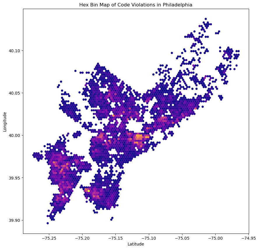
1.2.4 Spatially join data sets
To do a census tract comparison to our eviction data, we need to find which census tract each of the code violations falls into. Use the geopandas.sjoin() function to do just that.
Hints - You can re-use your eviction data frame, but you will only need the geometry column (specifying census tract polygons) and the GEOID column (specifying the name of each census tract). - Make sure both data frames have the same CRS before joining them together!
tidytractsNoDup = tidytracts.drop_duplicates("GEOID")
tidytractsNoDup| GEOID | geometry | year | evictions | |
|---|---|---|---|---|
| 0 | 42101000100 | MULTIPOLYGON (((-75.14161 39.95549, -75.14163 ... | e-03 | 21.0 |
| 1 | 42101000200 | MULTIPOLYGON (((-75.15122 39.95686, -75.15167 ... | e-03 | 3.0 |
| 2 | 42101000300 | MULTIPOLYGON (((-75.16234 39.95782, -75.16237 ... | e-03 | 17.0 |
| 3 | 42101000801 | MULTIPOLYGON (((-75.17732 39.95096, -75.17784 ... | e-03 | 13.0 |
| 4 | 42101000804 | MULTIPOLYGON (((-75.17118 39.94778, -75.17102 ... | e-03 | 21.0 |
| ... | ... | ... | ... | ... |
| 379 | 42101017800 | MULTIPOLYGON (((-75.11339 39.99649, -75.11137 ... | e-03 | 105.0 |
| 380 | 42101017900 | MULTIPOLYGON (((-75.10591 39.98804, -75.10836 ... | e-03 | 45.0 |
| 381 | 42101018002 | MULTIPOLYGON (((-75.10506 39.98707, -75.10437 ... | e-03 | 21.0 |
| 382 | 42101018300 | MULTIPOLYGON (((-75.06581 39.98629, -75.06859 ... | e-03 | 6.0 |
| 383 | 42101018400 | MULTIPOLYGON (((-75.05902 39.99251, -75.05954 ... | e-03 | 1.0 |
384 rows × 4 columns
violations.head()| lat | lng | violationdescription | geometry | |
|---|---|---|---|---|
| 2 | 40.050593 | -75.126578 | LICENSE-RES SFD/2FD | POINT (-75.12658 40.05059) |
| 25 | 40.022406 | -75.121872 | EXT S-ROOF REPAIR | POINT (-75.12187 40.02241) |
| 30 | 40.023237 | -75.121726 | CO DETECTOR NEEDED | POINT (-75.12173 40.02324) |
| 31 | 40.023397 | -75.122241 | INT S-CEILING REPAIR/MAINT SAN | POINT (-75.12224 40.02340) |
| 34 | 40.023773 | -75.121603 | INT S-FLOOR REPAIR | POINT (-75.12160 40.02377) |
tidytractsNoDup = tidytractsNoDup.to_crs("EPSG:4326")
violations = violations.to_crs("EPSG:4326")
joined_data = gpd.sjoin(violations, tidytractsNoDup)
joined_data| lat | lng | violationdescription | geometry | index_right | GEOID | year | evictions | |
|---|---|---|---|---|---|---|---|---|
| 2 | 40.050593 | -75.126578 | LICENSE-RES SFD/2FD | POINT (-75.12658 40.05059) | 364 | 42101027100 | e-03 | 6.0 |
| 16024 | 40.045785 | -75.127928 | CO DETECTOR NEEDED | POINT (-75.12793 40.04579) | 364 | 42101027100 | e-03 | 6.0 |
| 17225 | 40.045634 | -75.126469 | LICENSE-RES SFD/2FD | POINT (-75.12647 40.04563) | 364 | 42101027100 | e-03 | 6.0 |
| 43436 | 40.045738 | -75.125851 | INT S-CEILING REPAIR/MAINT SAN | POINT (-75.12585 40.04574) | 364 | 42101027100 | e-03 | 6.0 |
| 43452 | 40.045779 | -75.125843 | EXT S-ROOF REPAIR | POINT (-75.12584 40.04578) | 364 | 42101027100 | e-03 | 6.0 |
| ... | ... | ... | ... | ... | ... | ... | ... | ... |
| 219512 | 40.101835 | -75.045433 | DRAINAGE-DOWNSPOUT REPR/REPLC | POINT (-75.04543 40.10184) | 136 | 42101035602 | e-03 | 7.0 |
| 224788 | 40.004739 | -75.206722 | INT S-CEILING REPAIR/MAINT SAN | POINT (-75.20672 40.00474) | 283 | 42101012201 | e-03 | 28.0 |
| 224790 | 40.004739 | -75.206722 | INT S-CEILING REPAIR/MAINT SAN | POINT (-75.20672 40.00474) | 283 | 42101012201 | e-03 | 28.0 |
| 240195 | 40.013165 | -75.142804 | LICENSE-RES SFD/2FD | POINT (-75.14280 40.01317) | 171 | 42101980500 | e-03 | 0.0 |
| 310973 | 40.034424 | -75.017732 | DRAINAGE-DOWNSPOUT REPR/REPLC | POINT (-75.01773 40.03442) | 175 | 42101989100 | e-03 | 0.0 |
34108 rows × 8 columns
1.2.5 Calculate the number of violations by type per census tract
Next, we’ll want to find the number of violations (for each kind) per census tract. You should group the data frame by violation type and census tract name.
The result of this step should be a data frame with three columns: violationdescription, GEOID, and N, where N is the number of violations of that kind in the specified census tract.
Optional: to make prettier plots
Some census tracts won’t have any violations, and they won’t be included when we do the above calculation. However, there is a trick to set the values for those census tracts to be zero. After you calculate the sizes of each violation/census tract group, you can run:
N = N.unstack(fill_value=0).stack().reset_index(name='N')where N gives the total size of each of the groups, specified by violation type and census tract name.
See this StackOverflow post for more details.
This part is optional, but will make the resulting maps a bit prettier.
#N = N.unstack(fill_value=0).stack().reset_index(name='N')
violdesc = joined_data.groupby(["violationdescription", "GEOID"]).size().reset_index(name="N")
violdesc| violationdescription | GEOID | N | |
|---|---|---|---|
| 0 | CO DETECTOR NEEDED | 42101000401 | 1 |
| 1 | CO DETECTOR NEEDED | 42101000402 | 1 |
| 2 | CO DETECTOR NEEDED | 42101000700 | 1 |
| 3 | CO DETECTOR NEEDED | 42101000803 | 1 |
| 4 | CO DETECTOR NEEDED | 42101000804 | 1 |
| ... | ... | ... | ... |
| 3995 | VACANT PROPERTIES-GENERAL | 42101036501 | 1 |
| 3996 | VACANT PROPERTIES-GENERAL | 42101037900 | 1 |
| 3997 | VACANT PROPERTIES-GENERAL | 42101038000 | 1 |
| 3998 | VACANT PROPERTIES-GENERAL | 42101038200 | 2 |
| 3999 | VACANT PROPERTIES-GENERAL | 42101038300 | 3 |
4000 rows × 3 columns
1.2.6 Merge with census tracts geometries
We now have the number of violations of different types per census tract specified as a regular DataFrame. You can now merge it with the census tract geometries (from your eviction data GeoDataFrame) to create a GeoDataFrame.
Hints - Use pandas.merge() and specify the on keyword to be the column holding census tract names. - Make sure the result of the merge operation is a GeoDataFrame — you will want the GeoDataFrame holding census tract geometries to be the first argument of the pandas.merge() function.
mergedN_evics = tidytractsNoDup.merge(violdesc, on="GEOID")
mergedN_evics| GEOID | geometry | year | evictions | violationdescription | N | |
|---|---|---|---|---|---|---|
| 0 | 42101000100 | MULTIPOLYGON (((-75.14161 39.95549, -75.14163 ... | e-03 | 21.0 | DRAINAGE-DOWNSPOUT REPR/REPLC | 6 |
| 1 | 42101000100 | MULTIPOLYGON (((-75.14161 39.95549, -75.14163 ... | e-03 | 21.0 | ELECTRICAL -HAZARD | 1 |
| 2 | 42101000100 | MULTIPOLYGON (((-75.14161 39.95549, -75.14163 ... | e-03 | 21.0 | EXT S-ROOF REPAIR | 3 |
| 3 | 42101000100 | MULTIPOLYGON (((-75.14161 39.95549, -75.14163 ... | e-03 | 21.0 | INT S-CEILING REPAIR/MAINT SAN | 9 |
| 4 | 42101000100 | MULTIPOLYGON (((-75.14161 39.95549, -75.14163 ... | e-03 | 21.0 | INT S-FLOOR REPAIR | 2 |
| ... | ... | ... | ... | ... | ... | ... |
| 3995 | 42101018400 | MULTIPOLYGON (((-75.05902 39.99251, -75.05954 ... | e-03 | 1.0 | INT S-CEILING REPAIR/MAINT SAN | 4 |
| 3996 | 42101018400 | MULTIPOLYGON (((-75.05902 39.99251, -75.05954 ... | e-03 | 1.0 | INT S-FLOOR REPAIR | 2 |
| 3997 | 42101018400 | MULTIPOLYGON (((-75.05902 39.99251, -75.05954 ... | e-03 | 1.0 | INTERIOR SURFACES | 2 |
| 3998 | 42101018400 | MULTIPOLYGON (((-75.05902 39.99251, -75.05954 ... | e-03 | 1.0 | LICENSE-RES SFD/2FD | 11 |
| 3999 | 42101018400 | MULTIPOLYGON (((-75.05902 39.99251, -75.05954 ... | e-03 | 1.0 | PLUMBING SYSTEMS-GENERAL | 2 |
4000 rows × 6 columns
1.2.7 Interactive choropleths for each violation type
Now, we can use hvplot() to create an interactive choropleth for each violation type and add a widget to specify different violation types.
Hints - You’ll need to use the groupby keyword to tell hvplot to make a series of maps, with a widget to select different violation types. - You will need to specify dynamic=False as a keyword argument to the hvplot() function. - Be sure to specify a width and height that makes your output map (roughly) square to limit distortions
mergedN_evics.hvplot(
geo = True,
groupby = "violationdescription",
c = "N",
dynamic=False,
frame_width=600,
frame_height=600,
title="Evictions in Philadelphia by Year",
colormap="bmw"
)
1.3. A side-by-side comparison
From the interactive maps of evictions and violations, you should notice a lot of spatial overlap.
As a final step, we’ll make a side-by-side comparison to better show the spatial correlations. This will involve a few steps:
- Trim the evictions data frame plotted in section 1.1.5 to only include evictions from 2016.
- Trim the L+I violations data frame plotted in section 1.2.7 to only include a single violation type (pick whichever one you want!).
- Use
hvplot()to make two interactive choropleth maps, one for the data from step 1. and one for the data in step 2. - Show these two plots side by side (one row and 2 columns) using the syntax for combining charts.
Note: since we selected a single year and violation type, you won’t need to use the groupby= keyword here.
evics2016 = tidytracts[tidytracts["year"] == "e-16"]
evics2016| GEOID | geometry | year | evictions | |
|---|---|---|---|---|
| 4992 | 42101000100 | MULTIPOLYGON (((-75.14161 39.95549, -75.14163 ... | e-16 | 16.0 |
| 4993 | 42101000200 | MULTIPOLYGON (((-75.15122 39.95686, -75.15167 ... | e-16 | 8.0 |
| 4994 | 42101000300 | MULTIPOLYGON (((-75.16234 39.95782, -75.16237 ... | e-16 | 14.0 |
| 4995 | 42101000801 | MULTIPOLYGON (((-75.17732 39.95096, -75.17784 ... | e-16 | 4.0 |
| 4996 | 42101000804 | MULTIPOLYGON (((-75.17118 39.94778, -75.17102 ... | e-16 | 7.0 |
| ... | ... | ... | ... | ... |
| 5371 | 42101017800 | MULTIPOLYGON (((-75.11339 39.99649, -75.11137 ... | e-16 | 104.0 |
| 5372 | 42101017900 | MULTIPOLYGON (((-75.10591 39.98804, -75.10836 ... | e-16 | 80.0 |
| 5373 | 42101018002 | MULTIPOLYGON (((-75.10506 39.98707, -75.10437 ... | e-16 | 32.0 |
| 5374 | 42101018300 | MULTIPOLYGON (((-75.06581 39.98629, -75.06859 ... | e-16 | 7.0 |
| 5375 | 42101018400 | MULTIPOLYGON (((-75.05902 39.99251, -75.05954 ... | e-16 | 2.0 |
384 rows × 4 columns
evics2016drain = mergedN_evics[mergedN_evics["violationdescription"] == "DRAINAGE-DOWNSPOUT REPR/REPLC"]
evics2016drain| GEOID | geometry | year | evictions | violationdescription | N | |
|---|---|---|---|---|---|---|
| 0 | 42101000100 | MULTIPOLYGON (((-75.14161 39.95549, -75.14163 ... | e-03 | 21.0 | DRAINAGE-DOWNSPOUT REPR/REPLC | 6 |
| 8 | 42101000200 | MULTIPOLYGON (((-75.15122 39.95686, -75.15167 ... | e-03 | 3.0 | DRAINAGE-DOWNSPOUT REPR/REPLC | 1 |
| 14 | 42101000300 | MULTIPOLYGON (((-75.16234 39.95782, -75.16237 ... | e-03 | 17.0 | DRAINAGE-DOWNSPOUT REPR/REPLC | 2 |
| 29 | 42101001002 | MULTIPOLYGON (((-75.14919 39.94903, -75.14602 ... | e-03 | 16.0 | DRAINAGE-DOWNSPOUT REPR/REPLC | 3 |
| 38 | 42101001400 | MULTIPOLYGON (((-75.16558 39.94366, -75.16567 ... | e-03 | 30.0 | DRAINAGE-DOWNSPOUT REPR/REPLC | 3 |
| ... | ... | ... | ... | ... | ... | ... |
| 3946 | 42101017800 | MULTIPOLYGON (((-75.11339 39.99649, -75.11137 ... | e-03 | 105.0 | DRAINAGE-DOWNSPOUT REPR/REPLC | 14 |
| 3961 | 42101017900 | MULTIPOLYGON (((-75.10591 39.98804, -75.10836 ... | e-03 | 45.0 | DRAINAGE-DOWNSPOUT REPR/REPLC | 21 |
| 3975 | 42101018002 | MULTIPOLYGON (((-75.10506 39.98707, -75.10437 ... | e-03 | 21.0 | DRAINAGE-DOWNSPOUT REPR/REPLC | 4 |
| 3985 | 42101018300 | MULTIPOLYGON (((-75.06581 39.98629, -75.06859 ... | e-03 | 6.0 | DRAINAGE-DOWNSPOUT REPR/REPLC | 3 |
| 3993 | 42101018400 | MULTIPOLYGON (((-75.05902 39.99251, -75.05954 ... | e-03 | 1.0 | DRAINAGE-DOWNSPOUT REPR/REPLC | 5 |
311 rows × 6 columns
p1 = evics2016drain.hvplot(
values="N",
hover_cols=["N"],
dynamic=False,
frame_width=600,
frame_height=600,
hover_color="yellow",
title="Reported Drainage Damage in Households 2016",
colormap='Greens'
)
p1
p2 = evics2016.hvplot(
values="evictions",
hover_cols="evictions",
dynamic=False,
width=700,
height=700,
hover_color="yellow",
title="Evictions in Philadelphia 2016",
)
p2WARNING:param.main: values option not found for polygons plot with bokeh; similar options include: []
WARNING:param.main: values option not found for polygons plot with bokeh; similar options include: []1.4. Extra Credit
Identify the 20 most common types of violations within the time period of 2012 to 2016 and create a set of interactive choropleths similar to what was done in section 1.2.7.
Use this set of maps to identify 3 types of violations that don’t seem to have much spatial overlap with the number of evictions in the City.
#tracts12to16 = tidytracts[tidytracts["year"].astype(str).isin[f"e-{x:02d}" for x in range(12, 17)]]
#tidytracts12to16 = tidytracts[tidytracts["year"] == "e-16" or tidytracts["year"] == "e-15" or tidytracts["year"] == "e-14" or tidytracts["year"] == "e-13" or tidytracts["year"] == "e-13" or tidytracts["year"] == "e-12"]
value_vars = [f"e-{x:02d}" for x in range(12, 17)]
tidytracts12to16 = tracts_filtered.melt(id_vars=["GEOID", "geometry"], value_vars=value_vars)
tidytracts12to16.rename(columns={"variable": "year", "value": "evictions"}, inplace=True)
tidytracts12to16| GEOID | geometry | year | evictions | |
|---|---|---|---|---|
| 0 | 42101000100 | MULTIPOLYGON (((-75.14161 39.95549, -75.14163 ... | e-12 | 7.0 |
| 1 | 42101000200 | MULTIPOLYGON (((-75.15122 39.95686, -75.15167 ... | e-12 | 3.0 |
| 2 | 42101000300 | MULTIPOLYGON (((-75.16234 39.95782, -75.16237 ... | e-12 | 12.0 |
| 3 | 42101000801 | MULTIPOLYGON (((-75.17732 39.95096, -75.17784 ... | e-12 | 0.0 |
| 4 | 42101000804 | MULTIPOLYGON (((-75.17118 39.94778, -75.17102 ... | e-12 | 16.0 |
| ... | ... | ... | ... | ... |
| 1915 | 42101017800 | MULTIPOLYGON (((-75.11339 39.99649, -75.11137 ... | e-16 | 104.0 |
| 1916 | 42101017900 | MULTIPOLYGON (((-75.10591 39.98804, -75.10836 ... | e-16 | 80.0 |
| 1917 | 42101018002 | MULTIPOLYGON (((-75.10506 39.98707, -75.10437 ... | e-16 | 32.0 |
| 1918 | 42101018300 | MULTIPOLYGON (((-75.06581 39.98629, -75.06859 ... | e-16 | 7.0 |
| 1919 | 42101018400 | MULTIPOLYGON (((-75.05902 39.99251, -75.05954 ... | e-16 | 2.0 |
1920 rows × 4 columns
grouped_evics = mergedN_evics.groupby("violationdescription").size().reset_index(name="N")
tidyevics = grouped_evics.sort_values(by=["N"], ascending=False)
top20_violations = tidyevics.iloc[:20, 0] top20_violations6 INT S-CEILING REPAIR/MAINT SAN
11 LICENSE-RES SFD/2FD
5 EXT S-ROOF REPAIR
0 CO DETECTOR NEEDED
1 DRAINAGE-DOWNSPOUT REPR/REPLC
7 INT S-FLOOR REPAIR
2 DRAINAGE-MAIN DRAIN REPAIR-RES
8 INT-PLMBG FIXTURES-RES
9 INT-PLMBG MAINT FIXTURES-RES
12 LIGHT FIXTURE DEFECTIVE-RES
3 ELEC-RECEPTABLE DEFECTIVE-RES
10 INTERIOR SURFACES
13 PLUMBING SYSTEMS-GENERAL
4 ELECTRICAL -HAZARD
14 VACANT PROPERTIES-GENERAL
Name: violationdescription, dtype: objectCelingVio2016 = mergedN_evics[mergedN_evics["violationdescription"] == "INT S-CEILING REPAIR/MAINT SAN"]COVio2016= mergedN_evics[mergedN_evics["violationdescription"] == "CO DETECTOR NEEDED"]ElectricVio2016 = mergedN_evics[mergedN_evics["violationdescription"] == "ELECTRICAL -HAZARD"]ElectricVio2016.hvplot(
values="N",
hover_cols="N",
dynamic=False,
width=700,
height=700,
hover_color="yellow",
colormap="bmw",
title="Electrical Hazards 2016",
)WARNING:param.main: values option not found for polygons plot with bokeh; similar options include: []COVio2016.hvplot(
values="N",
hover_cols="N",
dynamic=False,
width=700,
height=700,
hover_color="yellow",
colormap="coolwarm",
title="Carbon Monoxide Detectors Needed in 2016",
)WARNING:param.main: values option not found for polygons plot with bokeh; similar options include: []CelingVio2016.hvplot(
values="N",
hover_cols="N",
dynamic=False,
width=700,
height=700,
hover_color="yellow",
colormap="fire",
title="Ceiling Repair Violations 2016",
)WARNING:param.main: values option not found for polygons plot with bokeh; similar options include: []Part 2: Exploring the NDVI in Philadelphia
In this part, we’ll explore the NDVI in Philadelphia a bit more. This part will include two parts:
- We’ll compare the median NDVI within the city limits and the immediate suburbs
- We’ll calculate the NDVI around street trees in the city.
2.1 Comparing the NDVI in the city and the suburbs
2.1.1 Load Landsat data for Philadelphia
Use rasterio to load the landsat data for Philadelphia (available in the “data/” folder)
landsat = rio.open("./Data/landsat8_philly.tif")
landsat<open DatasetReader name='./Data/landsat8_philly.tif' mode='r'>2.1.2 Separating the city from the suburbs
Create two polygon objects, one for the city limits and one for the suburbs. To calculate the suburbs polygon, we will take everything outside the city limits but still within the bounding box.
- The city limits are available in the “data/” folder.
- To calculate the suburbs polygon, the “envelope” attribute of the city limits geometry will be useful.
- You can use geopandas’ geometric manipulation functionality to calculate the suburbs polygon from the city limits polygon and the envelope polygon.
envelope = CityLimitsdf.geometry.envelope
suburbs = envelope - CityLimitsdf.geometry
suburbsC:\Users\Owner\AppData\Local\Temp\ipykernel_7664\3105865041.py:2: FutureWarning: '-' operator will be deprecated. Use the 'difference' method instead.
suburbs = envelope - CityLimitsdf.geometry0 MULTIPOLYGON (((-75.28031 39.86747, -75.28031 ...
dtype: geometryprint(landsat.crs.to_epsg())32618CityLimitsdf = CityLimitsdf.to_crs(32618)
suburbs = suburbs.to_crs(32618)suburbs.squeeze()
2.1.3 Mask and calculate the NDVI for the city and the suburbs
Using the two polygons from the last section, use rasterio’s mask functionality to create two masked arrays from the landsat data, one for the city and one for the suburbs.
For each masked array, calculate the NDVI.
from rasterio.mask import maskmaskedCity, mask_transformCity = mask(
dataset=landsat,
shapes=CityLimitsdf.geometry,
crop=True,
all_touched=True,
filled=False,
)
maskedSub, mask_transform = mask(
dataset=landsat,
shapes=suburbs.geometry,
crop=True,
all_touched=True,
filled=False,
)
redC = maskedCity[3]
nirC = maskedCity[4]
redS = maskedSub[3]
nirS = maskedSub[4]def calculate_NDVI(nir, red):
nir = nir.astype(float)
red = red.astype(float)
check = np.logical_and(red.mask == False, nir.mask == False)
ndvi = np.where(check, (nir - red) / (nir + red), np.nan)
return ndvi
NDVI_C = calculate_NDVI(nirC, redC)
NDVI_S = calculate_NDVI(nirS, redS)2.1.4 Calculate the median NDVI within the city and within the suburbs
- Calculate the median value from your NDVI arrays for the city and suburbs
- Numpy’s
nanmedianfunction will be useful for ignoring NaN elements - Print out the median values. Which has a higher NDVI: the city or suburbs?
city_ndvi_median = np.nanmedian(NDVI_C)
suburbs_ndvi_median = np.nanmedian(NDVI_S)
print(f"Median NDVI for the city: {city_ndvi_median}")
print(f"Median NDVI for the suburbs: {suburbs_ndvi_median}")Median NDVI for the city: 0.20268593532493442
Median NDVI for the suburbs: 0.374669586889207762.2 Calculating the NDVI for Philadelphia’s street treets
2.2.1 Load the street tree data
The data is available in the “data/” folder. It has been downloaded from OpenDataPhilly. It contains the locations of abot 2,500 street trees in Philadelphia.
pprTreePoints| objectid | fcode | geometry | |
|---|---|---|---|
| 0 | 1 | 3000 | POINT (-75.00538 40.06254) |
| 1 | 2 | 3000 | POINT (-75.12959 39.96692) |
| 2 | 3 | 3000 | POINT (-75.12838 39.98397) |
| 3 | 4 | 3000 | POINT (-75.12892 39.98489) |
| 4 | 5 | 3000 | POINT (-75.12948 39.97148) |
| ... | ... | ... | ... |
| 2475 | 2476 | 3000 | POINT (-75.15779 39.97728) |
| 2476 | 2477 | 3000 | POINT (-75.15773 39.97727) |
| 2477 | 2478 | 3000 | POINT (-75.15768 39.97727) |
| 2478 | 2479 | 3000 | POINT (-75.15763 39.97725) |
| 2479 | 2480 | 3000 | POINT (-75.15757 39.97725) |
2480 rows × 3 columns
pprTreePoints = pprTreePoints.to_crs(32618)2.2.2 Calculate the NDVI values at the locations of the street trees
- Use the rasterstats package to calculate the NDVI values at the locations of the street trees.
- Since these are point geometries, you can calculate either the median or the mean statistic (only one pixel will contain each point).
import rasterstats
from rasterstats import zonal_statsstats = zonal_stats(
pprTreePoints, # The vector data
NDVI_C, # The array holding the raster data
affine=landsat.transform, # The affine transform for the raster data
stats=["mean", "median"], # The stats to compute
nodata=np.nan, # Missing data representation
)
#stats2.2.3 Plotting the results
Make two plots of the results:
- A histogram of the NDVI values, using matplotlib’s
histfunction. Include a vertical line that marks the NDVI = 0 threshold - A plot of the street tree points, colored by the NDVI value, using geopandas’
plotfunction. Include the city limits boundary on your plot.
The figures should be clear and well-styled, with for example, labels for axes, legends, and clear color choices.
median_stats = [stats_dict["median"] for stats_dict in stats]
mean_stats = [stats_dict["mean"] for stats_dict in stats]a2 = plt.subplots()
plt.hist(mean_stats, bins=100, density=True)
plt.axvline(0, linestyle="dashed", color="gray")
plt.xlabel("mean")
plt.ylabel("median")
plt.title("Histogram of NDVI Values for Street Trees in Philadelphia")
plt.grid(True)
plt.show()
a2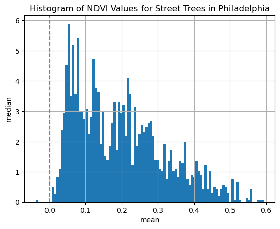
(<Figure size 640x480 with 1 Axes>,
<Axes: title={'center': 'Histogram of NDVI Values for Street Trees in Philadelphia'}, xlabel='mean', ylabel='median'>)pprTreePoints["median_stats"] = [stats_dict["median"] for stats_dict in stats]
pprTreePoints.head()| objectid | fcode | geometry | median_stats | |
|---|---|---|---|---|
| 0 | 1 | 3000 | POINT (499541.269 4434698.265) | 0.235337 |
| 1 | 2 | 3000 | POINT (488932.471 4424093.158) | 0.261535 |
| 2 | 3 | 3000 | POINT (489039.214 4425985.827) | 0.096769 |
| 3 | 4 | 3000 | POINT (488993.171 4426088.005) | 0.076630 |
| 4 | 5 | 3000 | POINT (488943.113 4424599.478) | 0.267952 |
pprTreePoints.explore(column="median_stats", cmap="magma", tiles="Cartodb positron")Make this Notebook Trusted to load map: File -> Trust Notebook